10 💻 PCA

⚠️ Note on Slides: If you encounter broken links in the PDF slides (module_2_PCA_&_CA.pdf), please refer to the “Online Resources and References” section at the end of this chapter for updated and working links.

10.1 Introduction to Principal Component Analysis

Principal Component Analysis (PCA) is a powerful dimensionality reduction technique used to transform a large set of variables into a smaller set of uncorrelated variables called principal components. These components capture the maximum variance in the data while reducing complexity.

10.1.1 Key Concepts

Dimensionality Reduction: Reduce the number of variables while retaining most of the information
Variance Preservation: Principal components are ordered by the amount of variance they explain
Uncorrelated Components: Each principal component is orthogonal (uncorrelated) to the others
Data Standardization: Often necessary when variables are on different scales

10.1.2 When to Use PCA

When you have many correlated variables
To visualize high-dimensional data in 2D or 3D
To reduce noise in the data
Before applying other machine learning algorithms
To identify the most important features in your dataset

10.2 Required Packages

We will use the following packages throughout this chapter:

library(FactoMineR)  # For PCA analysis
library(factoextra)  # For visualization
library(ISLR2)       # For datasets

10.3 17.1 PCA with FactoMineR Package

10.3.1 17.1.1 Example 1: Simple 2D Dataset

Let’s start with a simple example to understand the fundamentals of PCA.

10.3.1.1 Step 1: Create and Explore the Data

X <- data.frame(
  Var1 = c(2, 1, -1, -2),
  Var2 = c(2, -1, 1, -2)
)
rownames(X) <- c("i1", "i2", "i3", "i4")
X
#>    Var1 Var2
#> i1    2    2
#> i2    1   -1
#> i3   -1    1
#> i4   -2   -2

10.3.1.2 Step 2: Calculate Covariance Matrix and Inertia

# Calculate means
mean(X[,1]) # mean of Var1
#> [1] 0
mean(X[,2]) # mean of Var2
#> [1] 0

# Variance-covariance matrix
# The constant (n-1)/n adjusts for the variance-covariance matrix used in lectures
S <- var(X) * (3/4)
S
#>      Var1 Var2
#> Var1  2.5  1.5
#> Var2  1.5  2.5

# Inertia (sum of diagonal elements = sum of variances)
Inertia <- sum(diag(S))
Inertia
#> [1] 5

10.3.1.3 Step 3: Eigen-analysis on Covariance Matrix

eigen(S) # gives the eigen-values and eigen-vectors
#> eigen() decomposition
#> $values
#> [1] 4 1
#> 
#> $vectors
#>           [,1]       [,2]
#> [1,] 0.7071068 -0.7071068
#> [2,] 0.7071068  0.7071068

10.3.1.4 Step 4: Eigen-analysis on Correlation Matrix

# Correlation matrix
R <- cor(X)
eigenan <- eigen(R) # eigen analysis of R
eigenan
#> eigen() decomposition
#> $values
#> [1] 1.6 0.4
#> 
#> $vectors
#>           [,1]       [,2]
#> [1,] 0.7071068 -0.7071068
#> [2,] 0.7071068  0.7071068

# Sum of eigenvalues equals p (number of variables)
sum(eigenan$values)
#> [1] 2

# Normalized data (centered and scaled)
Z <- scale(X)
var(Z) # is the correlation matrix
#>      Var1 Var2
#> Var1  1.0  0.6
#> Var2  0.6  1.0

10.3.1.5 Step 5: Perform PCA on Covariance Matrix

PCA with the covariance matrix uses only centered data. For PCA on the correlation matrix (normed PCA), use scale.unit = TRUE (default option).

Note on Correlation: The correlation between two variables $X_1$ and $X_2$ is: \[\rho = \frac{cov(X_1, X_2)}{\sigma_{X_1} \sigma_{X_2}}\]

where $cov(X_1, X_2)$ is the covariance, and $\sigma_{X_1} = \sqrt{Var(X_1)}$ is the standard deviation of $X_1$.

res.pca.cov <- PCA(X, scale.unit = FALSE, graph = FALSE)
print(res.pca.cov)
#> **Results for the Principal Component Analysis (PCA)**
#> The analysis was performed on 4 individuals, described by 2 variables
#> *The results are available in the following objects:
#> 
#>    name               description                          
#> 1  "$eig"             "eigenvalues"                        
#> 2  "$var"             "results for the variables"          
#> 3  "$var$coord"       "coord. for the variables"           
#> 4  "$var$cor"         "correlations variables - dimensions"
#> 5  "$var$cos2"        "cos2 for the variables"             
#> 6  "$var$contrib"     "contributions of the variables"     
#> 7  "$ind"             "results for the individuals"        
#> 8  "$ind$coord"       "coord. for the individuals"         
#> 9  "$ind$cos2"        "cos2 for the individuals"           
#> 10 "$ind$contrib"     "contributions of the individuals"   
#> 11 "$call"            "summary statistics"                 
#> 12 "$call$centre"     "mean of the variables"              
#> 13 "$call$ecart.type" "standard error of the variables"    
#> 14 "$call$row.w"      "weights for the individuals"        
#> 15 "$call$col.w"      "weights for the variables"

10.3.1.6 Step 6: Examine Eigenvalues

We have $p = 2 = min(n-1, p) = min(3, 2)$ eigenvalues: 4 and 1. The inertia $Inertia = 4 + 1 = 5$ is the sum of the variances of the variables.

res.pca.cov$eig
#>        eigenvalue percentage of variance
#> comp 1          4                     80
#> comp 2          1                     20
#>        cumulative percentage of variance
#> comp 1                                80
#> comp 2                               100

10.3.1.7 Step 7: Examine Variables and Individuals

res.pca.cov$var
#> $coord
#>         Dim.1      Dim.2
#> Var1 1.414214 -0.7071068
#> Var2 1.414214  0.7071068
#> 
#> $cor
#>          Dim.1      Dim.2
#> Var1 0.8944272 -0.4472136
#> Var2 0.8944272  0.4472136
#> 
#> $cos2
#>      Dim.1 Dim.2
#> Var1   0.8   0.2
#> Var2   0.8   0.2
#> 
#> $contrib
#>      Dim.1 Dim.2
#> Var1    50    50
#> Var2    50    50

res.pca.cov$ind
#> $coord
#>                         Dim.1                       Dim.2
#> i1  2.82842712474619073503845 -0.000000000000000006357668
#> i2  0.00000000000000001271534 -1.414213562373095367519227
#> i3 -0.00000000000000040992080  1.414213562373094923430017
#> i4 -2.82842712474619029094924  0.000000000000000204960400
#> 
#> $cos2
#>                                          Dim.1
#> i1 1.00000000000000044408920985006261616945267
#> i2 0.00000000000000000000000000000000008083988
#> i3 0.00000000000000000000000000000008401753104
#> i4 1.00000000000000022204460492503130808472633
#>                                           Dim.2
#> i1 0.000000000000000000000000000000000005052492
#> i2 1.000000000000000444089209850062616169452667
#> i3 0.999999999999999777955395074968691915273666
#> i4 0.000000000000000000000000000000005251095690
#> 
#> $contrib
#>                                         Dim.1
#> i1 50.000000000000021316282072803005576133728
#> i2  0.000000000000000000000000000000001010498
#> i3  0.000000000000000000000000000001050219138
#> i4 50.000000000000014210854715202003717422485
#>                                         Dim.2
#> i1  0.000000000000000000000000000000001010498
#> i2 50.000000000000021316282072803005576133728
#> i3 49.999999999999985789145284797996282577515
#> i4  0.000000000000000000000000000001050219138
#> 
#> $dist
#>       i1       i2       i3       i4 
#> 2.828427 1.414214 1.414214 2.828427

10.3.2 17.1.2 Example 2: Student Grades Dataset

Now let’s work with a more realistic example: student grades in three subjects.

10.3.2.1 Step 1: Prepare the Data

A <- matrix(c(9,12,10,15,9,10,5,10,8,11,13,14,11,13,8,3,15,10), 
            nrow=6, byrow=TRUE)
A
#>      [,1] [,2] [,3]
#> [1,]    9   12   10
#> [2,]   15    9   10
#> [3,]    5   10    8
#> [4,]   11   13   14
#> [5,]   11   13    8
#> [6,]    3   15   10

Nframe <- as.data.frame(A)

# Set row and column names
m1 <- c("Alex", "Bea", "Claudio", "Damien", "Emilie", "Fran")
m2 <- c("Biostatistics", "Economics", "English")

rownames(A) <- m1
colnames(A) <- m2
head(A)
#>         Biostatistics Economics English
#> Alex                9        12      10
#> Bea                15         9      10
#> Claudio             5        10       8
#> Damien             11        13      14
#> Emilie             11        13       8
#> Fran                3        15      10

10.3.2.2 Step 2: Perform PCA on Correlation Matrix

res.pca.cor <- PCA(A, scale.unit = TRUE, graph = FALSE)
print(res.pca.cor)
#> **Results for the Principal Component Analysis (PCA)**
#> The analysis was performed on 6 individuals, described by 3 variables
#> *The results are available in the following objects:
#> 
#>    name               description                          
#> 1  "$eig"             "eigenvalues"                        
#> 2  "$var"             "results for the variables"          
#> 3  "$var$coord"       "coord. for the variables"           
#> 4  "$var$cor"         "correlations variables - dimensions"
#> 5  "$var$cos2"        "cos2 for the variables"             
#> 6  "$var$contrib"     "contributions of the variables"     
#> 7  "$ind"             "results for the individuals"        
#> 8  "$ind$coord"       "coord. for the individuals"         
#> 9  "$ind$cos2"        "cos2 for the individuals"           
#> 10 "$ind$contrib"     "contributions of the individuals"   
#> 11 "$call"            "summary statistics"                 
#> 12 "$call$centre"     "mean of the variables"              
#> 13 "$call$ecart.type" "standard error of the variables"    
#> 14 "$call$row.w"      "weights for the individuals"        
#> 15 "$call$col.w"      "weights for the variables"

10.3.2.3 Step 3: Examine Eigenvalues

res.pca.cor$eig
#>        eigenvalue percentage of variance
#> comp 1  1.5000000               50.00000
#> comp 2  1.1830127               39.43376
#> comp 3  0.3169873               10.56624
#>        cumulative percentage of variance
#> comp 1                          50.00000
#> comp 2                          89.43376
#> comp 3                         100.00000
get_eigenvalue(res.pca.cor)
#>       eigenvalue variance.percent
#> Dim.1  1.5000000         50.00000
#> Dim.2  1.1830127         39.43376
#> Dim.3  0.3169873         10.56624
#>       cumulative.variance.percent
#> Dim.1                    50.00000
#> Dim.2                    89.43376
#> Dim.3                   100.00000

Interpretation: Kaiser’s rule suggests $q = 2$ components because the eigenvalue mean is 1 (with 89% of explained variance). The rule of thumb gives $q = 2$ because the first 2 dimensions explain 89% of the variance/inertia.

10.3.2.4 Step 4: Examine Variables

res.pca.cor$var
#> $coord
#>                                  Dim.1     Dim.2      Dim.3
#> Biostatistics -0.866025403784438041477 0.3535534  0.3535534
#> Economics      0.866025403784439040678 0.3535534  0.3535534
#> English        0.000000000000001047394 0.9659258 -0.2588190
#> 
#> $cor
#>                                  Dim.1     Dim.2      Dim.3
#> Biostatistics -0.866025403784438041477 0.3535534  0.3535534
#> Economics      0.866025403784439151700 0.3535534  0.3535534
#> English        0.000000000000001047394 0.9659258 -0.2588190
#> 
#> $cos2
#>                                                Dim.1
#> Biostatistics 0.749999999999999000799277837359113619
#> Economics     0.750000000000000888178419700125232339
#> English       0.000000000000000000000000000001097035
#>                   Dim.2     Dim.3
#> Biostatistics 0.1250000 0.1250000
#> Economics     0.1250000 0.1250000
#> English       0.9330127 0.0669873
#> 
#> $contrib
#>                                                Dim.1
#> Biostatistics 49.99999999999993605115378159098327160
#> Economics     50.00000000000005684341886080801486969
#> English        0.00000000000000000000000000007313567
#>                  Dim.2    Dim.3
#> Biostatistics 10.56624 39.43376
#> Economics     10.56624 39.43376
#> English       78.86751 21.13249

10.3.2.5 Step 5: Correlations Between Variables and Components

res.pca.cor$var$cor
#>                                  Dim.1     Dim.2      Dim.3
#> Biostatistics -0.866025403784438041477 0.3535534  0.3535534
#> Economics      0.866025403784439151700 0.3535534  0.3535534
#> English        0.000000000000001047394 0.9659258 -0.2588190

Interpretation: The first axis is correlated with Biostatistics (+0.86) and Economics (-0.86). The second axis is correlated to English (0.96). The two components are correlated with at least one variable, so $q = 2$ may be considered to reduce the dimension from $p = 3$.

10.3.2.6 Step 6: Coordinates of Variables

res.pca.cor$var$coord
#>                                  Dim.1     Dim.2      Dim.3
#> Biostatistics -0.866025403784438041477 0.3535534  0.3535534
#> Economics      0.866025403784439040678 0.3535534  0.3535534
#> English        0.000000000000001047394 0.9659258 -0.2588190

10.3.2.7 Step 7: Quality of Representation (cos²)

res.pca.cor$var$cos2
#>                                                Dim.1
#> Biostatistics 0.749999999999999000799277837359113619
#> Economics     0.750000000000000888178419700125232339
#> English       0.000000000000000000000000000001097035
#>                   Dim.2     Dim.3
#> Biostatistics 0.1250000 0.1250000
#> Economics     0.1250000 0.1250000
#> English       0.9330127 0.0669873

Interpretation: Biostatistics and Economics are well represented in the first dimension (75%), while English is very well represented in the second axis (93%). In the first plane (Dim.1 and Dim.2), Biostatistics and Economics are well represented (75% + 12.5% = 87.5%), and English is very well represented (93% + 0% = 93%).

10.3.2.8 Step 8: Contributions of Variables

res.pca.cor$var$contrib
#>                                                Dim.1
#> Biostatistics 49.99999999999993605115378159098327160
#> Economics     50.00000000000005684341886080801486969
#> English        0.00000000000000000000000000007313567
#>                  Dim.2    Dim.3
#> Biostatistics 10.56624 39.43376
#> Economics     10.56624 39.43376
#> English       78.86751 21.13249

Interpretation: Biostatistics and Economics contribute to the construction of the first dimension (50%), while English contributes highly to the construction of the second axis (78.8%). In the first plane, the contribution of Biostatistics and Economics is 50% + 10.5% = 60.5%, and that of English is 78.8%.

10.3.2.9 Step 9: Description of Dimensions

dimdesc(res.pca.cor, axes = 1)
#> $Dim.1
#> 
#> Link between the variable and the continuous variables (R-square)
#> =================================================================================
#>               correlation    p.value
#> Economics       0.8660254 0.02572142
#> Biostatistics  -0.8660254 0.02572142

10.3.2.10 Step 10: Contributions of First Two Dimensions

res.pca.cor$var$contrib[, 1:2]
#>                                                Dim.1
#> Biostatistics 49.99999999999993605115378159098327160
#> Economics     50.00000000000005684341886080801486969
#> English        0.00000000000000000000000000007313567
#>                  Dim.2
#> Biostatistics 10.56624
#> Economics     10.56624
#> English       78.86751

10.3.3 17.1.3 Visualizations

10.3.3.1 Variables Plot

fviz_pca_var(res.pca.cor, col.var = "black")

10.3.3.2 Variables Plot with Quality of Representation

fviz_pca_var(res.pca.cor, col.var = "cos2",
             gradient.cols = c("#00AFBB", "#E7B800", "#FC4E07"),
             repel = TRUE)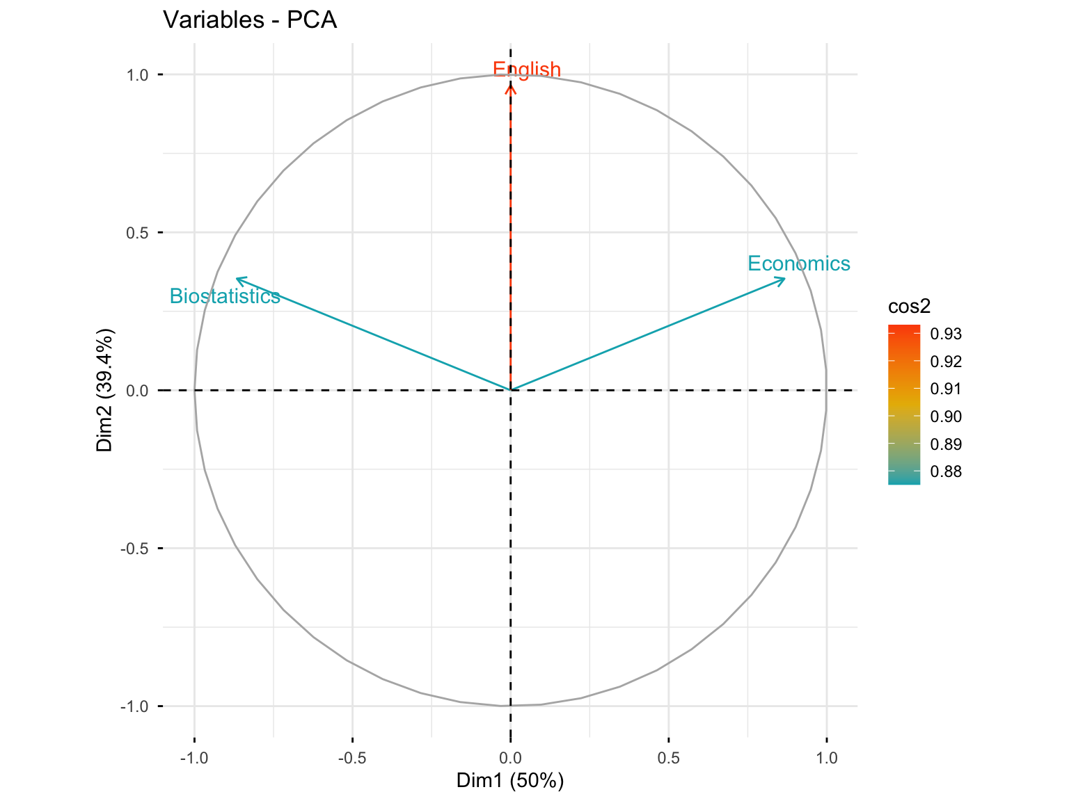

10.3.3.3 Variables with High Quality of Representation (cos² > 0.6)

fviz_pca_var(res.pca.cor, select.var = list(cos2 = 0.6))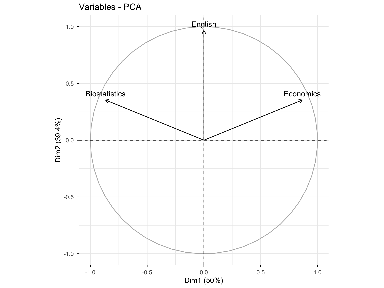

10.3.3.4 Variables Plot with Contributions

fviz_pca_var(res.pca.cor, col.var = "contrib",
             gradient.cols = c("#00AFBB", "#E7B800", "#FC4E07"))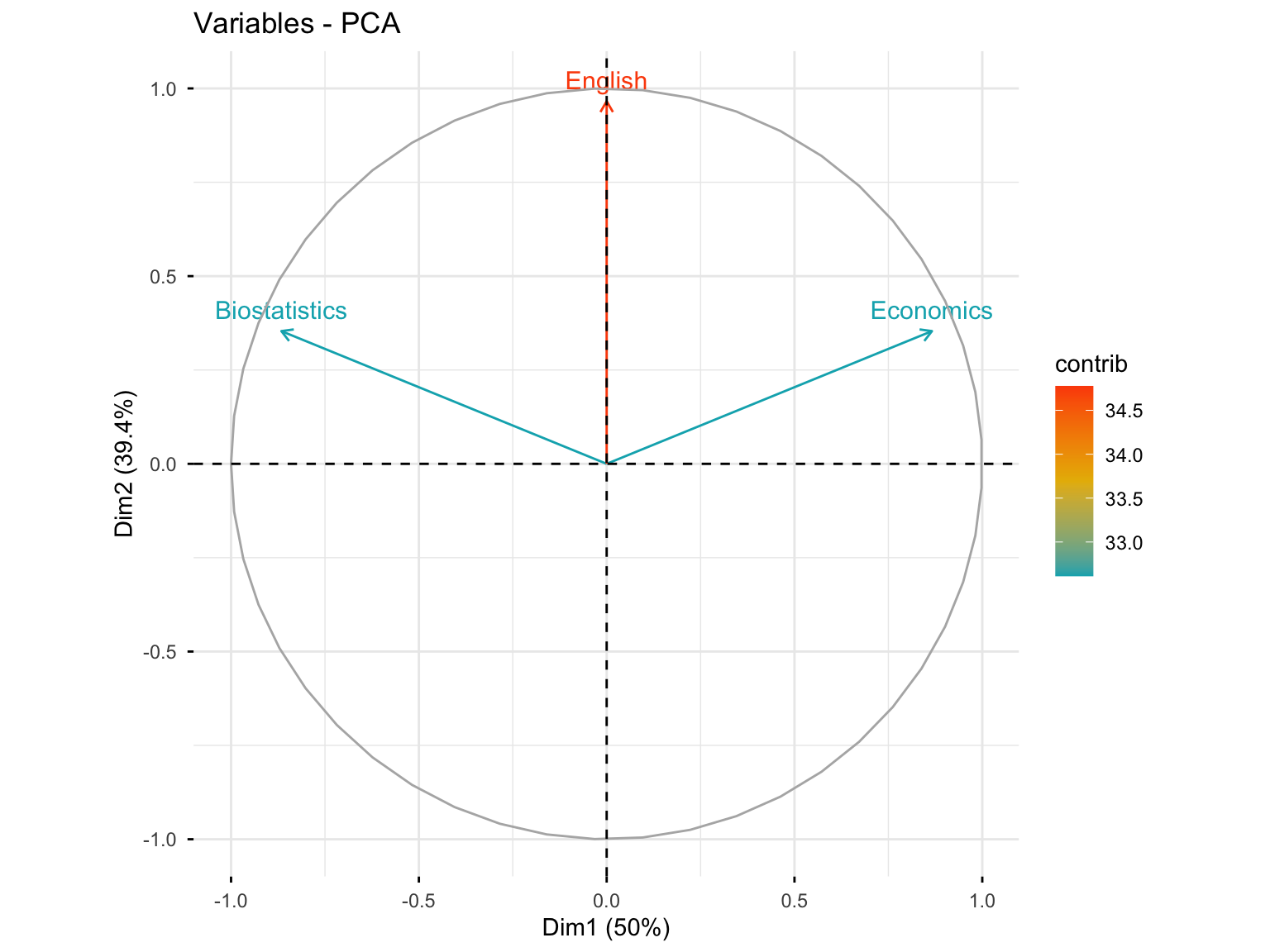

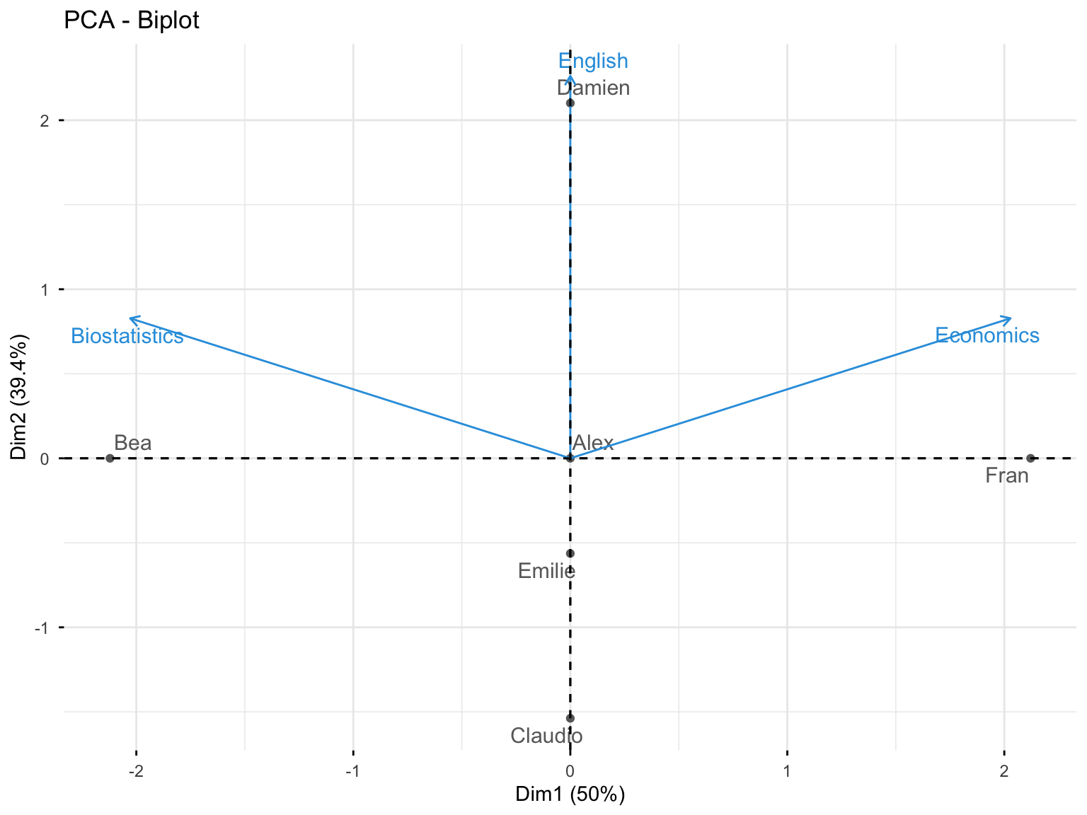
10.3.3.5 Biplot: Variables and Individuals

fviz_pca_biplot(res.pca.cor, repel = TRUE,
                col.var = "#2E9FDF", # Variables color
                col.ind = "#696969"  # Individuals color
)

10.3.4 17.1.4 Analysis of Individuals

10.3.4.1 Individuals Information

res.pca.cor$ind
#> $coord
#>                             Dim.1                    Dim.2
#> Alex     0.0000000000000002653034 -0.000000000000000941663
#> Bea     -2.1213203435596423851450  0.000000000000001237395
#> Claudio -0.0000000000000022171779 -1.538189001320852344890
#> Damien   0.0000000000000026937746  2.101205251626097503248
#> Emilie   0.0000000000000001895371 -0.563016250305248155961
#> Fran     2.1213203435596428292342 -0.000000000000002975084
#>                              Dim.3
#> Alex    -0.00000000000000007994654
#> Bea      0.00000000000000015526499
#> Claudio -0.79622521701812609684623
#> Damien  -0.29143865656241157990891
#> Emilie   1.08766387358053817635550
#> Fran     0.00000000000000002468473
#> 
#> $cos2
#>                                            Dim.1
#> Alex    0.07137976857538211317155685264879139140
#> Bea     1.00000000000000022204460492503130808473
#> Claudio 0.00000000000000000000000000000163862588
#> Damien  0.00000000000000000000000000000161253810
#> Emilie  0.00000000000000000000000000000002394954
#> Fran    0.99999999999999977795539507496869191527
#>                                           Dim.2
#> Alex    0.8992501752497785716400358069222420454
#> Bea     0.0000000000000000000000000000003402549
#> Claudio 0.7886751345948129765517364830884616822
#> Damien  0.9811252243246878501636842884181533009
#> Emilie  0.2113248654051877173376539076343760826
#> Fran    0.0000000000000000000000000000019669168
#>                                             Dim.3
#> Alex    0.006481699860810073883510273873298501712
#> Bea     0.000000000000000000000000000000005357159
#> Claudio 0.211324865405187134470565979427192360163
#> Damien  0.018874775675311854933324795524640649091
#> Emilie  0.788675134594813309618643870635423809290
#> Fran    0.000000000000000000000000000000000135408
#> 
#> $contrib
#>                                            Dim.1
#> Alex     0.0000000000000000000000000000007820654
#> Bea     50.0000000000000000000000000000000000000
#> Claudio  0.0000000000000000000000000000546208628
#> Damien   0.0000000000000000000000000000806269052
#> Emilie   0.0000000000000000000000000000003991590
#> Fran    50.0000000000000213162820728030055761337
#>                                          Dim.2
#> Alex     0.00000000000000000000000000001249253
#> Bea      0.00000000000000000000000000002157130
#> Claudio 33.33333333333337833437326480634510517
#> Damien  62.20084679281458051036679535172879696
#> Emilie   4.46581987385206335972043234505690634
#> Fran     0.00000000000000000000000000012469753
#>                                             Dim.3
#> Alex     0.00000000000000000000000000000033605182
#> Bea      0.00000000000000000000000000000126751744
#> Claudio 33.33333333333333570180911920033395290375
#> Damien   4.46581987385203582618942164117470383644
#> Emilie  62.20084679281465867006772896274924278259
#> Fran     0.00000000000000000000000000000003203788
#> 
#> $dist
#>                     Alex                      Bea 
#> 0.0000000000000009930137 2.1213203435596419410558 
#>                  Claudio                   Damien 
#> 1.7320508075688780813550 2.1213203435596419410558 
#>                   Emilie                     Fran 
#> 1.2247448713915896068016 2.1213203435596428292342

10.3.4.2 Individuals: Coordinates

res.pca.cor$ind$coord
#>                             Dim.1                    Dim.2
#> Alex     0.0000000000000002653034 -0.000000000000000941663
#> Bea     -2.1213203435596423851450  0.000000000000001237395
#> Claudio -0.0000000000000022171779 -1.538189001320852344890
#> Damien   0.0000000000000026937746  2.101205251626097503248
#> Emilie   0.0000000000000001895371 -0.563016250305248155961
#> Fran     2.1213203435596428292342 -0.000000000000002975084
#>                              Dim.3
#> Alex    -0.00000000000000007994654
#> Bea      0.00000000000000015526499
#> Claudio -0.79622521701812609684623
#> Damien  -0.29143865656241157990891
#> Emilie   1.08766387358053817635550
#> Fran     0.00000000000000002468473

10.3.4.3 Individuals: Quality of Representation

res.pca.cor$ind$cos2
#>                                            Dim.1
#> Alex    0.07137976857538211317155685264879139140
#> Bea     1.00000000000000022204460492503130808473
#> Claudio 0.00000000000000000000000000000163862588
#> Damien  0.00000000000000000000000000000161253810
#> Emilie  0.00000000000000000000000000000002394954
#> Fran    0.99999999999999977795539507496869191527
#>                                           Dim.2
#> Alex    0.8992501752497785716400358069222420454
#> Bea     0.0000000000000000000000000000003402549
#> Claudio 0.7886751345948129765517364830884616822
#> Damien  0.9811252243246878501636842884181533009
#> Emilie  0.2113248654051877173376539076343760826
#> Fran    0.0000000000000000000000000000019669168
#>                                             Dim.3
#> Alex    0.006481699860810073883510273873298501712
#> Bea     0.000000000000000000000000000000005357159
#> Claudio 0.211324865405187134470565979427192360163
#> Damien  0.018874775675311854933324795524640649091
#> Emilie  0.788675134594813309618643870635423809290
#> Fran    0.000000000000000000000000000000000135408

10.3.4.4 Individuals: Contributions

res.pca.cor$ind$contrib
#>                                            Dim.1
#> Alex     0.0000000000000000000000000000007820654
#> Bea     50.0000000000000000000000000000000000000
#> Claudio  0.0000000000000000000000000000546208628
#> Damien   0.0000000000000000000000000000806269052
#> Emilie   0.0000000000000000000000000000003991590
#> Fran    50.0000000000000213162820728030055761337
#>                                          Dim.2
#> Alex     0.00000000000000000000000000001249253
#> Bea      0.00000000000000000000000000002157130
#> Claudio 33.33333333333337833437326480634510517
#> Damien  62.20084679281458051036679535172879696
#> Emilie   4.46581987385206335972043234505690634
#> Fran     0.00000000000000000000000000012469753
#>                                             Dim.3
#> Alex     0.00000000000000000000000000000033605182
#> Bea      0.00000000000000000000000000000126751744
#> Claudio 33.33333333333333570180911920033395290375
#> Damien   4.46581987385203582618942164117470383644
#> Emilie  62.20084679281465867006772896274924278259
#> Fran     0.00000000000000000000000000000003203788

10.3.4.5 Individuals Plot with Contributions

fviz_pca_ind(res.pca.cor, col.ind = "contrib",
             gradient.cols = c("#00AFBB", "#E7B800", "#FC4E07"))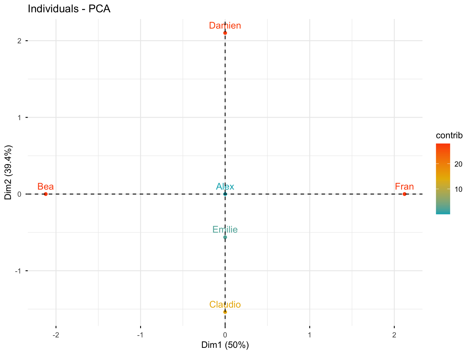

10.3.4.6 Individuals Plot with Quality of Representation

fviz_pca_ind(res.pca.cor, col.ind = "cos2",
             gradient.cols = c("#00AFBB", "#E7B800", "#FC4E07"),
             repel = TRUE)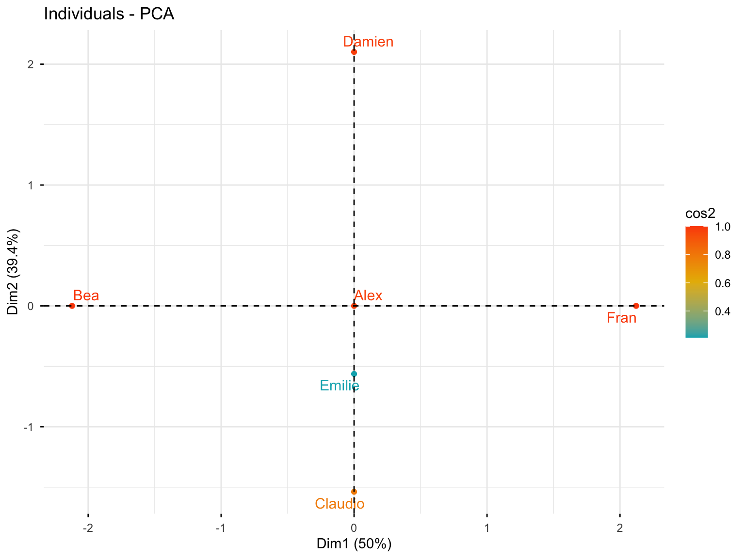

10.3.5 17.1.5 Exporting Results

10.3.5.1 Save Figures as PDF

pdf("PCA.pdf")
fviz_pca_var(res.pca.cor)
fviz_pca_ind(res.pca.cor)
dev.off()

10.3.5.2 Save Figures as PNG

png("PCA%03d.png", width = 800, height = 600)
fviz_pca_var(res.pca.cor)
fviz_pca_ind(res.pca.cor)
dev.off()

10.3.5.3 Export Results to Text Files

write.table(res.pca.cor$eig, "eigenvalues.txt", sep = "\t")
write.table(res.pca.cor$var$coord, "variables_coordinates.txt", sep = "\t")
write.table(res.pca.cor$ind$coord, "individuals_coordinates.txt", sep = "\t")

10.4 17.2 PCA with Base R: prcomp() Function

The prcomp() function is part of base R and provides an alternative way to perform PCA. Let’s use the USArrests dataset, which contains crime statistics for the 50 US states.

10.4.1 17.2.1 Data Exploration

# Load and examine the data
head(USArrests)
#>            Murder Assault UrbanPop Rape
#> Alabama      13.2     236       58 21.2
#> Alaska       10.0     263       48 44.5
#> Arizona       8.1     294       80 31.0
#> Arkansas      8.8     190       50 19.5
#> California    9.0     276       91 40.6
#> Colorado      7.9     204       78 38.7
rownames(USArrests)
#>  [1] "Alabama"        "Alaska"         "Arizona"       
#>  [4] "Arkansas"       "California"     "Colorado"      
#>  [7] "Connecticut"    "Delaware"       "Florida"       
#> [10] "Georgia"        "Hawaii"         "Idaho"         
#> [13] "Illinois"       "Indiana"        "Iowa"          
#> [16] "Kansas"         "Kentucky"       "Louisiana"     
#> [19] "Maine"          "Maryland"       "Massachusetts" 
#> [22] "Michigan"       "Minnesota"      "Mississippi"   
#> [25] "Missouri"       "Montana"        "Nebraska"      
#> [28] "Nevada"         "New Hampshire"  "New Jersey"    
#> [31] "New Mexico"     "New York"       "North Carolina"
#> [34] "North Dakota"   "Ohio"           "Oklahoma"      
#> [37] "Oregon"         "Pennsylvania"   "Rhode Island"  
#> [40] "South Carolina" "South Dakota"   "Tennessee"     
#> [43] "Texas"          "Utah"           "Vermont"       
#> [46] "Virginia"       "Washington"     "West Virginia" 
#> [49] "Wisconsin"      "Wyoming"

The dataset contains four variables:

Murder: Murder arrests (per 100,000)
Assault: Assault arrests (per 100,000)
UrbanPop: Percent urban population
Rape: Rape arrests (per 100,000)

colnames(USArrests)
#> [1] "Murder"   "Assault"  "UrbanPop" "Rape"

10.4.2 17.2.2 Data Preprocessing: Why Standardization Matters

Notice that the variables have vastly different means. The apply() function with option 2 calculates statistics for each column (option 1 does it by row):

apply(USArrests, 2, mean)
#>   Murder  Assault UrbanPop     Rape 
#>    7.788  170.760   65.540   21.232

There are on average three times as many rapes as murders, and more than eight times as many assaults as rapes. Let’s examine the variances:

apply(USArrests, 2, var)
#>     Murder    Assault   UrbanPop       Rape 
#>   18.97047 6945.16571  209.51878   87.72916

Important: The variables have very different variances. The UrbanPop variable (percentage) is not comparable to the number of arrests per 100,000. If we don’t scale the variables before performing PCA, most principal components would be driven by the Assault variable, since it has the largest mean and variance. It is crucial to standardize variables to have mean zero and standard deviation one before performing PCA.

10.4.3 17.2.3 Performing PCA with prcomp()

The option scale = TRUE scales the variables to have standard deviation one.

pr.out <- prcomp(USArrests, scale = TRUE)
names(pr.out)
#> [1] "sdev"     "rotation" "center"   "scale"    "x"

The center and scale components correspond to the means and standard deviations used for scaling:

pr.out$center
#>   Murder  Assault UrbanPop     Rape 
#>    7.788  170.760   65.540   21.232
pr.out$scale
#>    Murder   Assault  UrbanPop      Rape 
#>  4.355510 83.337661 14.474763  9.366385

10.4.4 17.2.4 Principal Component Loadings

The rotation matrix provides the principal component loadings; each column contains the corresponding principal component loading vector.

pr.out$rotation
#>                 PC1        PC2        PC3         PC4
#> Murder   -0.5358995  0.4181809 -0.3412327  0.64922780
#> Assault  -0.5831836  0.1879856 -0.2681484 -0.74340748
#> UrbanPop -0.2781909 -0.8728062 -0.3780158  0.13387773
#> Rape     -0.5434321 -0.1673186  0.8177779  0.08902432

We see that there are four distinct principal components. This is expected because there are generally $min(n-1, p)$ informative principal components in a dataset with $n$ observations and $p$ variables.

10.4.5 17.2.5 Principal Component Scores

Using pr.out$x, we have the $50 \times 4$ matrix of principal component score vectors. The $k$th column is the $k$th principal component score vector.

dim(pr.out$x)
#> [1] 50  4
head(pr.out$x)
#>                   PC1        PC2         PC3          PC4
#> Alabama    -0.9756604  1.1220012 -0.43980366  0.154696581
#> Alaska     -1.9305379  1.0624269  2.01950027 -0.434175454
#> Arizona    -1.7454429 -0.7384595  0.05423025 -0.826264240
#> Arkansas    0.1399989  1.1085423  0.11342217 -0.180973554
#> California -2.4986128 -1.5274267  0.59254100 -0.338559240
#> Colorado   -1.4993407 -0.9776297  1.08400162  0.001450164

10.4.6 17.2.6 Visualizing Results

We can plot the first two principal components as follows:

biplot(pr.out, scale = 0)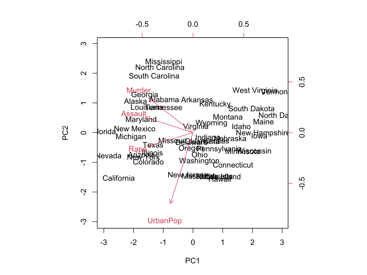

The scale = 0 argument ensures that the arrows are scaled to represent the loadings; other values give slightly different biplots with different interpretations.

Note: Principal components are only unique up to a sign change. We can reproduce the figure by changing signs:

pr.out$rotation <- -pr.out$rotation
pr.out$x <- -pr.out$x
biplot(pr.out, scale = 0)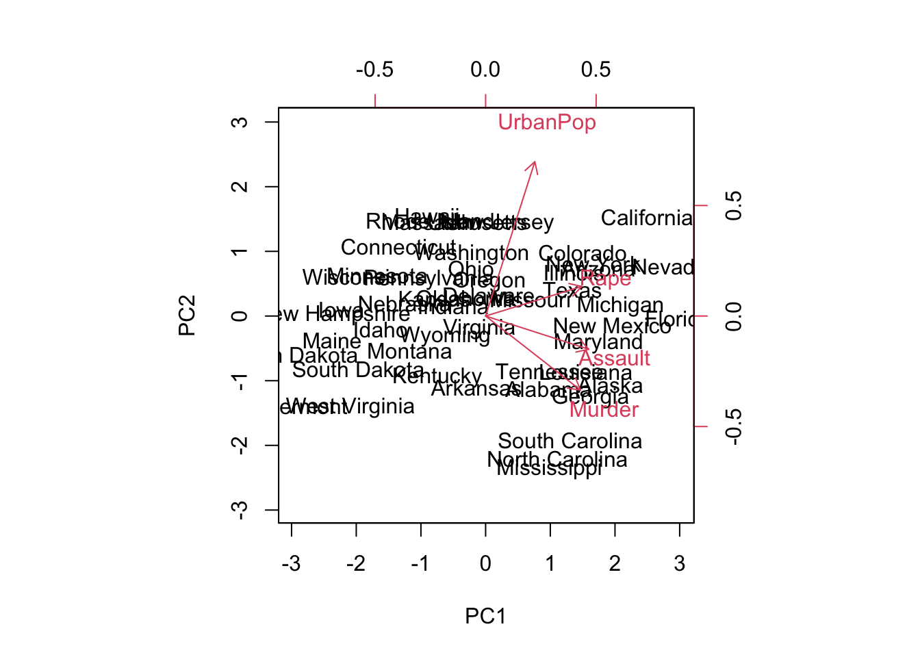

10.4.7 17.2.7 Variance Explained

The standard deviation (square root of the corresponding eigenvalue) of each principal component:

pr.out$sdev
#> [1] 1.5748783 0.9948694 0.5971291 0.4164494

The variance explained by each principal component (corresponding eigenvalue) is obtained by squaring these:

pr.var <- pr.out$sdev^2
pr.var
#> [1] 2.4802416 0.9897652 0.3565632 0.1734301

Compute the proportion of variance explained by each principal component:

pve <- pr.var / sum(pr.var)
pve
#> [1] 0.62006039 0.24744129 0.08914080 0.04335752

We see that the first principal component explains 62.0% of the variance, and the next explains 24.7%. Let’s plot the PVE (Proportion of Variance Explained) and cumulative PVE:

par(mfrow = c(1, 2))
plot(pve, xlab = "Principal Component", 
     ylab = "Proportion of Variance Explained", 
     ylim = c(0, 1), type = "b")
plot(cumsum(pve), xlab = "Principal Component", 
     ylab = "Cumulative Proportion of Variance Explained", 
     ylim = c(0, 1), type = "b")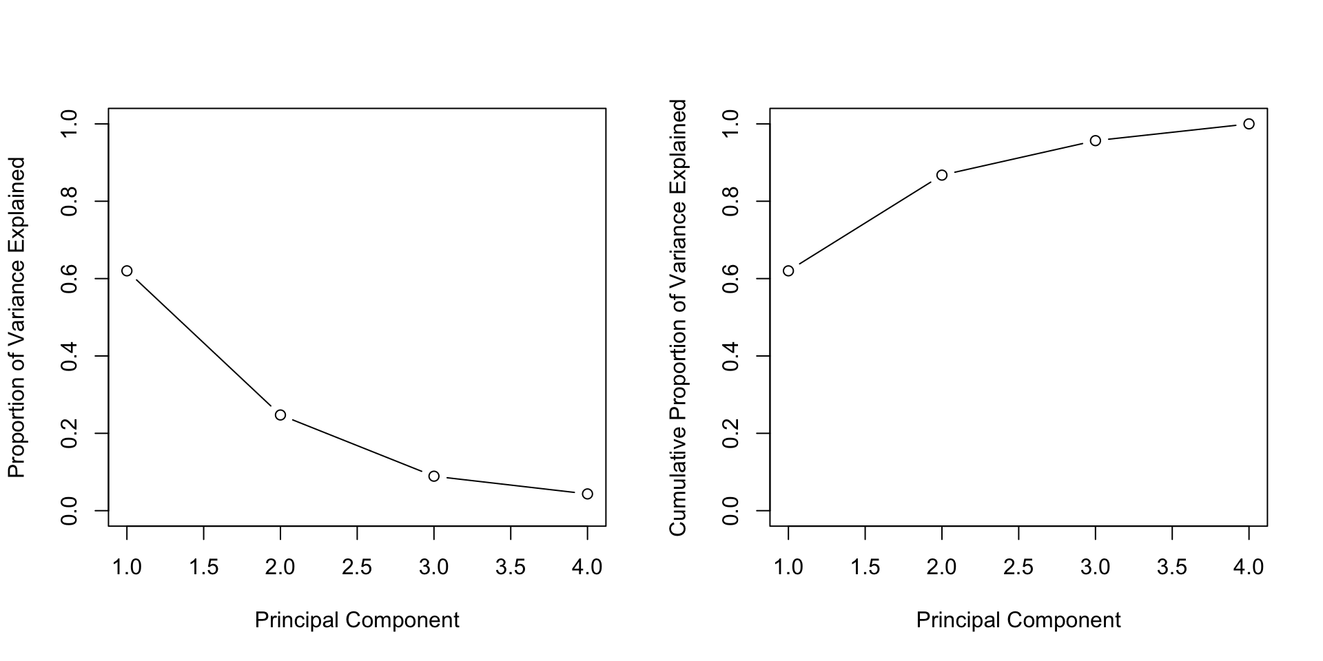

par(mfrow = c(1, 1))

The function cumsum() computes the cumulative sum of the elements of a numeric vector.

10.5 17.3 Practical Exercises

10.5.1 Exercise 1: US Cereals Dataset

Consider the UScereal dataset from the MASS package (65 rows and 11 columns), which contains nutritional and marketing information from the 1993 ASA Statistical Graphics Exposition. The data have been normalized to a portion of one American cup.

Tasks:

Load the dataset and examine its structure
Identify which variables are quantitative and suitable for PCA
Perform PCA on the quantitative variables
Interpret the results: how many components should be retained?
Create visualizations to understand the relationships between variables

library(MASS)
data(UScereal)
# Note: Some variables are not quantitative
# Select only quantitative variables before performing PCA
# res.pca.cereal <- PCA(UScereal[, quantitative_cols], scale.unit = TRUE, graph = FALSE)

10.5.2 Exercise 2: NCI Cancer Cell Line Data

Consider the NCI cancer cell line microarray data from ISLR2, which consists of 6,830 gene expression measurements on 64 cancer cell lines.

Tasks:

Load the dataset
Perform PCA on the gene expression data
Visualize the first few principal components
Check if the cancer types (given in nci.labs) cluster together in the PCA space

library(ISLR2)
data(NCI60)
# Each cell line is labeled with a cancer type, given in nci.labs
# Perform PCA and check if cancer types cluster in the first two dimensions

10.5.3 Exercise 3: Wine Quality Analysis

Consider the wine dataset from the gclus package, which contains chemical analyses of wines grown in the same region in Italy but derived from three different cultivars. The dataset has 13 variables and over 170 observations.

Tasks:

Perform PCA on the wine dataset. Remember to standardize the variables as they are on different scales.

library(gclus)
data(wine)
library(FactoMineR)
# Perform PCA
res.pca.wine <- PCA(wine, scale.unit = TRUE, graph = FALSE)

Interpret the PCA results. Focus on:

Which chemical properties contribute most to the variance?
Do the wines cluster by cultivar?
How many principal components should be retained?

10.5.4 Exercise 4: Boston Housing Data

Consider the Boston dataset from the MASS package, which contains information collected by the U.S. Census Service concerning housing in the area of Boston, Massachusetts. It has 506 rows and 14 columns.

Tasks:

Conduct PCA on the Boston housing dataset. Before performing PCA:

Assess which variables are most suitable for the analysis
Handle any missing values
Preprocess the data accordingly

library(MASS)
data(Boston)
library(FactoMineR)
# Select appropriate variables and perform PCA
res.pca.boston <- PCA(Boston, scale.unit = TRUE, graph = FALSE)

Interpret the results. Look for patterns indicating relationships between:

Crime rates
Property tax
Median value of owner-occupied homes
Other housing characteristics

10.5.5 General Guidelines for Solving Exercises

Data Preprocessing: Before performing PCA, it’s crucial to:
- Handle missing values appropriately
- Standardize the data (especially when variables are on different scales)
- Select relevant quantitative variables
PCA Interpretation: When interpreting results, focus on:
- Eigenvalues and proportion of variance explained
- Loadings of variables on principal components
- Quality of representation (cos²)
- Contributions of variables and individuals
Visualization: Use plots to aid interpretation:
- Scree plots (eigenvalues)
- Biplots (variables and individuals together)
- Variable plots (with contributions or quality)
- Individual plots
Contextual Understanding: Understanding the domain context can significantly help in interpreting results meaningfully. Always relate statistical findings back to the real-world problem you’re solving.

10.6 Online Resources and References

10.6.1 Official Documentation

FactoMineR Package:
factoextra Package:
- CRAN page
- Documentation

10.6.2 R Markdown Resources (as mentioned in slides)

R Markdown Cheat Sheet: RStudio Cheatsheets - Download the R Markdown cheat sheet
R Markdown Guide: R Markdown: The Definitive Guide
RStudio: Download RStudio
R Markdown Tutorial: R Markdown Tutorial

10.6.3 Tutorials and Guides

PCA Tutorial: STHDA - Principal Component Analysis in R
CA Tutorial: STHDA - Correspondence Analysis in R
R-bloggers: Search for PCA and CA articles at R-bloggers.com

10.6.4 Interactive Tools

PCA Visualization: PCA Explorer - Interactive PCA visualization tool
R Documentation: rdocumentation.org - Search for PCA and CA functions

10.6.5 Books and Academic Resources

An Introduction to Applied Multivariate Analysis with R by Everitt & Hothorn
Principal Component Analysis by Jolliffe (classic textbook)
Correspondence Analysis in Practice by Greenacre

10.6.6 Quick Reference

FactoMineR Help: Type ?PCA or ?CA in R console after loading the package
factoextra Help: Type ?fviz_pca_var or ?fviz_ca_biplot in R console

⚠️ Important: If you encounter broken links in the PDF slides (module_2_PCA_&_CA.pdf), all the links above are verified and working. Use this section as your reference for online resources.

9 🚀 Advanced Modeling Techniques

11 💻 Lab: PCA & Correspondence Analysis