11 💻 Lab: PCA & Correspondence Analysis
⚠️ Note on Slides: If you encounter broken links in the PDF slides (
module_2_PCA_&_CA.pdf), please refer to the “Additional Resources” section at the end of this lab for updated and working links.
This is a hands-on laboratory session to practice Principal Component Analysis (PCA) and Correspondence Analysis (CA) after the theoretical lecture. Work through these exercises step by step, and don’t hesitate to ask questions!
11.1 Setup
First, load the required packages:
library(FactoMineR)  # For PCA and CA
library(factoextra)  # For visualization
library(corrplot)    # For correlation plots
library(dplyr)       # For data manipulation
11.2 Part 1: Principal Component Analysis (PCA)
11.2.1 Exercise 1.1: Understanding the Data - Wine Dataset
We’ll work with the wine dataset from the gclus package, which contains chemical analyses of wines from three different cultivars.
# Load the wine dataset
library(gclus)
#> Caricamento del pacchetto richiesto: cluster
data(wine)

# Examine the structure
str(wine)
#> 'data.frame':    178 obs. of  14 variables:
#>  $ Class          : num  1 1 1 1 1 1 1 1 1 1 ...
#>  $ Alcohol        : num  14.2 13.2 13.2 14.4 13.2 ...
#>  $ Malic          : num  1.71 1.78 2.36 1.95 2.59 1.76 1.87 2.15 1.64 1.35 ...
#>  $ Ash            : num  2.43 2.14 2.67 2.5 2.87 2.45 2.45 2.61 2.17 2.27 ...
#>  $ Alcalinity     : num  15.6 11.2 18.6 16.8 21 15.2 14.6 17.6 14 16 ...
#>  $ Magnesium      : num  127 100 101 113 118 112 96 121 97 98 ...
#>  $ Phenols        : num  2.8 2.65 2.8 3.85 2.8 3.27 2.5 2.6 2.8 2.98 ...
#>  $ Flavanoids     : num  3.06 2.76 3.24 3.49 2.69 3.39 2.52 2.51 2.98 3.15 ...
#>  $ Nonflavanoid   : num  0.28 0.26 0.3 0.24 0.39 0.34 0.3 0.31 0.29 0.22 ...
#>  $ Proanthocyanins: num  2.29 1.28 2.81 2.18 1.82 1.97 1.98 1.25 1.98 1.85 ...
#>  $ Intensity      : num  5.64 4.38 5.68 7.8 4.32 6.75 5.25 5.05 5.2 7.22 ...
#>  $ Hue            : num  1.04 1.05 1.03 0.86 1.04 1.05 1.02 1.06 1.08 1.01 ...
#>  $ OD280          : num  3.92 3.4 3.17 3.45 2.93 2.85 3.58 3.58 2.85 3.55 ...
#>  $ Proline        : num  1065 1050 1185 1480 735 ...
head(wine)
#>   Class Alcohol Malic  Ash Alcalinity Magnesium Phenols
#> 1     1   14.23  1.71 2.43       15.6       127    2.80
#> 2     1   13.20  1.78 2.14       11.2       100    2.65
#> 3     1   13.16  2.36 2.67       18.6       101    2.80
#> 4     1   14.37  1.95 2.50       16.8       113    3.85
#> 5     1   13.24  2.59 2.87       21.0       118    2.80
#> 6     1   14.20  1.76 2.45       15.2       112    3.27
#>   Flavanoids Nonflavanoid Proanthocyanins Intensity  Hue
#> 1       3.06         0.28            2.29      5.64 1.04
#> 2       2.76         0.26            1.28      4.38 1.05
#> 3       3.24         0.30            2.81      5.68 1.03
#> 4       3.49         0.24            2.18      7.80 0.86
#> 5       2.69         0.39            1.82      4.32 1.04
#> 6       3.39         0.34            1.97      6.75 1.05
#>   OD280 Proline
#> 1  3.92    1065
#> 2  3.40    1050
#> 3  3.17    1185
#> 4  3.45    1480
#> 5  2.93     735
#> 6  2.85    1450
dim(wine)
#> [1] 178  14

# Check for missing values
sum(is.na(wine))
#> [1] 0
Questions: 1. How many observations and variables are in the dataset? 2. What types of variables do we have? 3. Are there any missing values?
11.2.2 Exercise 1.2: Data Exploration and Preprocessing
Before performing PCA, let’s explore the data and understand why standardization is important.
# Calculate means for each variable
apply(wine, 2, mean)
#>           Class         Alcohol           Malic
#>       1.9382022      13.0006180       2.3363483
#>             Ash      Alcalinity       Magnesium
#>       2.3665169      19.4949438      99.7415730
#>         Phenols      Flavanoids    Nonflavanoid
#>       2.2951124       2.0292697       0.3618539
#> Proanthocyanins       Intensity             Hue
#>       1.5908989       5.0580899       0.9574719
#>           OD280         Proline
#>       2.6116854     746.8932584

# Calculate variances for each variable
apply(wine, 2, var)
#>           Class         Alcohol           Malic
#>      0.60067924      0.65906233      1.24801540
#>             Ash      Alcalinity       Magnesium
#>      0.07526464     11.15268616    203.98933536
#>         Phenols      Flavanoids    Nonflavanoid
#>      0.39168954      0.99771867      0.01548863
#> Proanthocyanins       Intensity             Hue
#>      0.32759467      5.37444944      0.05224273
#>           OD280         Proline
#>      0.50408641  99166.71735542

# Calculate standard deviations
apply(wine, 2, sd)
#>           Class         Alcohol           Malic
#>       0.7750350       0.8118265       1.1171461
#>             Ash      Alcalinity       Magnesium
#>       0.2743440       3.3395638      14.2824835
#>         Phenols      Flavanoids    Nonflavanoid
#>       0.6258510       0.9988587       0.1244533
#> Proanthocyanins       Intensity             Hue
#>       0.5723589       2.3182859       0.2285667
#>           OD280         Proline
#>       0.7099904     314.9074743

# Create a correlation matrix
cor_matrix <- cor(wine)
cor_matrix
#>                       Class     Alcohol       Malic
#> Class            1.00000000 -0.32822194  0.43777620
#> Alcohol         -0.32822194  1.00000000  0.09439694
#> Malic            0.43777620  0.09439694  1.00000000
#> Ash             -0.04964322  0.21154460  0.16404547
#> Alcalinity       0.51785911 -0.31023514  0.28850040
#> Magnesium       -0.20917939  0.27079823 -0.05457510
#> Phenols         -0.71916334  0.28910112 -0.33516700
#> Flavanoids      -0.84749754  0.23681493 -0.41100659
#> Nonflavanoid     0.48910916 -0.15592947  0.29297713
#> Proanthocyanins -0.49912982  0.13669791 -0.22074619
#> Intensity        0.26566757  0.54636419  0.24898534
#> Hue             -0.61737454 -0.07183528 -0.56137198
#> OD280           -0.78822959  0.07234319 -0.36871043
#> Proline         -0.63371678  0.64372004 -0.19201056
#>                          Ash  Alcalinity   Magnesium
#> Class           -0.049643221  0.51785911 -0.20917939
#> Alcohol          0.211544596 -0.31023514  0.27079823
#> Malic            0.164045470  0.28850040 -0.05457510
#> Ash              1.000000000  0.44336719  0.28658669
#> Alcalinity       0.443367187  1.00000000 -0.08333309
#> Magnesium        0.286586691 -0.08333309  1.00000000
#> Phenols          0.128979538 -0.32111332  0.21440123
#> Flavanoids       0.115077279 -0.35136986  0.19578377
#> Nonflavanoid     0.186230446  0.36192172 -0.25629405
#> Proanthocyanins  0.009651935 -0.19732684  0.23644061
#> Intensity        0.258887257  0.01873198  0.19995000
#> Hue             -0.074724894 -0.27393429  0.05542194
#> OD280            0.003911231 -0.27676855  0.06600394
#> Proline          0.223626264 -0.44059693  0.39335085
#>                     Phenols Flavanoids Nonflavanoid
#> Class           -0.71916334 -0.8474975    0.4891092
#> Alcohol          0.28910112  0.2368149   -0.1559295
#> Malic           -0.33516700 -0.4110066    0.2929771
#> Ash              0.12897954  0.1150773    0.1862304
#> Alcalinity      -0.32111332 -0.3513699    0.3619217
#> Magnesium        0.21440123  0.1957838   -0.2562940
#> Phenols          1.00000000  0.8645635   -0.4499353
#> Flavanoids       0.86456350  1.0000000   -0.5378996
#> Nonflavanoid    -0.44993530 -0.5378996    1.0000000
#> Proanthocyanins  0.61241308  0.6526918   -0.3658451
#> Intensity       -0.05513642 -0.1723794    0.1390570
#> Hue              0.43350181  0.5433903   -0.2626388
#> OD280            0.69994936  0.7871939   -0.5032696
#> Proline          0.49811488  0.4941931   -0.3113852
#>                 Proanthocyanins   Intensity         Hue
#> Class              -0.499129824  0.26566757 -0.61737454
#> Alcohol             0.136697912  0.54636419 -0.07183528
#> Malic              -0.220746187  0.24898534 -0.56137198
#> Ash                 0.009651935  0.25888726 -0.07472489
#> Alcalinity         -0.197326836  0.01873198 -0.27393429
#> Magnesium           0.236440610  0.19995000  0.05542194
#> Phenols             0.612413084 -0.05513642  0.43350181
#> Flavanoids          0.652691769 -0.17237940  0.54339029
#> Nonflavanoid       -0.365845099  0.13905701 -0.26263878
#> Proanthocyanins     1.000000000 -0.02524993  0.29552796
#> Intensity          -0.025249935  1.00000000 -0.52191000
#> Hue                 0.295527964 -0.52191000  1.00000000
#> OD280               0.519067096 -0.42881494  0.56537014
#> Proline             0.330416700  0.31610011  0.23622715
#>                        OD280    Proline
#> Class           -0.788229589 -0.6337168
#> Alcohol          0.072343187  0.6437200
#> Malic           -0.368710428 -0.1920106
#> Ash              0.003911231  0.2236263
#> Alcalinity      -0.276768549 -0.4405969
#> Magnesium        0.066003936  0.3933508
#> Phenols          0.699949365  0.4981149
#> Flavanoids       0.787193902  0.4941931
#> Nonflavanoid    -0.503269596 -0.3113852
#> Proanthocyanins  0.519067096  0.3304167
#> Intensity       -0.428814943  0.3161001
#> Hue              0.565370143  0.2362272
#> OD280            1.000000000  0.3127611
#> Proline          0.312761075  1.0000000

# Visualize correlations
corrplot(cor_matrix, method = "circle", type = "upper",
         order = "hclust", tl.cex = 0.8)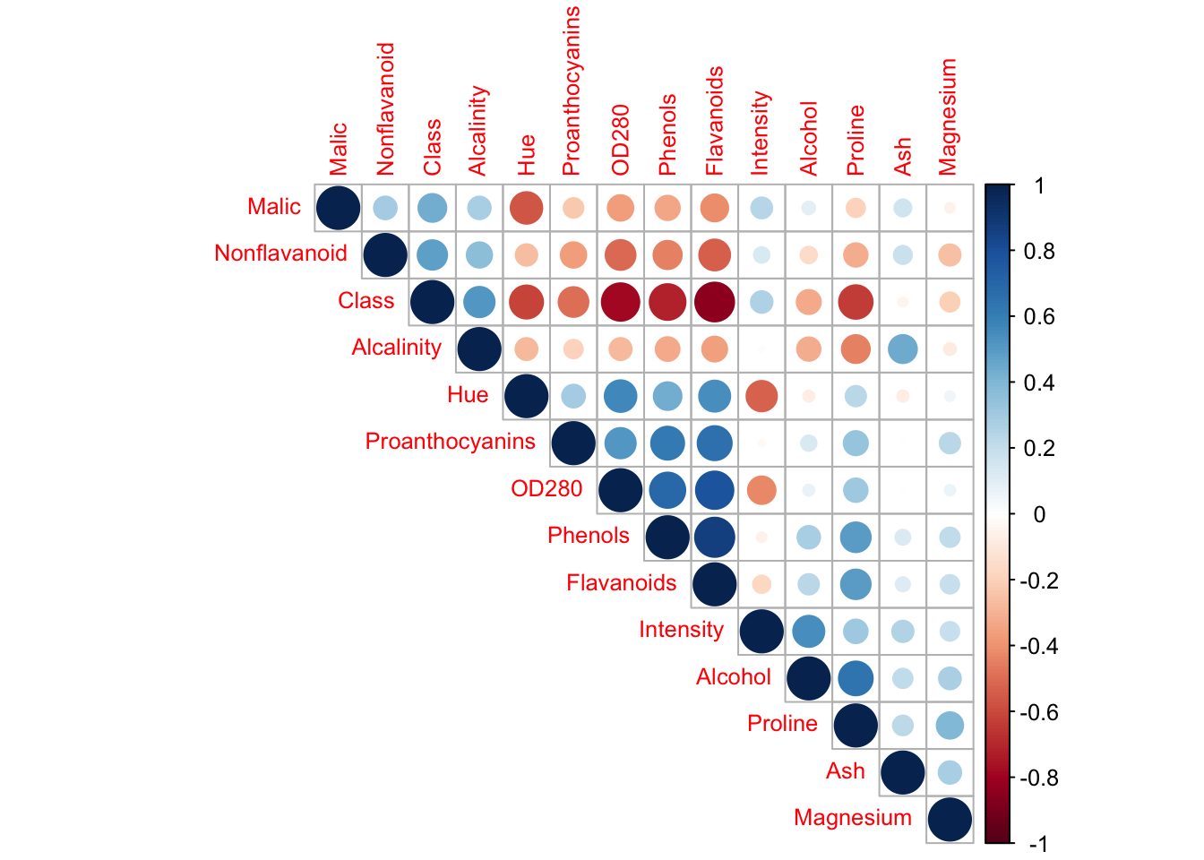
Questions: 1. Do the variables have similar scales? Why is this important for PCA? 2. Which variables are highly correlated? What does this suggest? 3. Should we standardize the data? Why or why not?
11.2.3 Exercise 1.3: Perform PCA
Now let’s perform PCA on the wine dataset.
# Perform PCA with standardization
res.pca.wine <- PCA(wine, scale.unit = TRUE, graph = FALSE)

# Print summary
print(res.pca.wine)
#> **Results for the Principal Component Analysis (PCA)**
#> The analysis was performed on 178 individuals, described by 14 variables
#> *The results are available in the following objects:
#>
#>    name               description
#> 1  "$eig"             "eigenvalues"
#> 2  "$var"             "results for the variables"
#> 3  "$var$coord"       "coord. for the variables"
#> 4  "$var$cor"         "correlations variables - dimensions"
#> 5  "$var$cos2"        "cos2 for the variables"
#> 6  "$var$contrib"     "contributions of the variables"
#> 7  "$ind"             "results for the individuals"
#> 8  "$ind$coord"       "coord. for the individuals"
#> 9  "$ind$cos2"        "cos2 for the individuals"
#> 10 "$ind$contrib"     "contributions of the individuals"
#> 11 "$call"            "summary statistics"
#> 12 "$call$centre"     "mean of the variables"
#> 13 "$call$ecart.type" "standard error of the variables"
#> 14 "$call$row.w"      "weights for the individuals"
#> 15 "$call$col.w"      "weights for the variables"
Questions: 1. How many principal components were created? 2. Why is this number equal to the number of variables (or n-1)?
11.2.4 Exercise 1.4: Examine Eigenvalues
# Get eigenvalues
eigenvalues <- get_eigenvalue(res.pca.wine)
eigenvalues
#>        eigenvalue variance.percent
#> Dim.1  5.53588574       39.5420410
#> Dim.2  2.49713353       17.8366681
#> Dim.3  1.44606409       10.3290292
#> Dim.4  0.92800966        6.6286404
#> Dim.5  0.87749595        6.2678282
#> Dim.6  0.67277837        4.8055598
#> Dim.7  0.55380907        3.9557791
#> Dim.8  0.35009358        2.5006684
#> Dim.9  0.29448553        2.1034681
#> Dim.10 0.26225251        1.8732322
#> Dim.11 0.22584552        1.6131823
#> Dim.12 0.16877391        1.2055279
#> Dim.13 0.12956002        0.9254287
#> Dim.14 0.05781251        0.4129465
#>        cumulative.variance.percent
#> Dim.1                     39.54204
#> Dim.2                     57.37871
#> Dim.3                     67.70774
#> Dim.4                     74.33638
#> Dim.5                     80.60421
#> Dim.6                     85.40977
#> Dim.7                     89.36555
#> Dim.8                     91.86621
#> Dim.9                     93.96968
#> Dim.10                    95.84291
#> Dim.11                    97.45610
#> Dim.12                    98.66162
#> Dim.13                    99.58705
#> Dim.14                   100.00000

# Alternative way
res.pca.wine$eig
#>         eigenvalue percentage of variance
#> comp 1  5.53588574             39.5420410
#> comp 2  2.49713353             17.8366681
#> comp 3  1.44606409             10.3290292
#> comp 4  0.92800966              6.6286404
#> comp 5  0.87749595              6.2678282
#> comp 6  0.67277837              4.8055598
#> comp 7  0.55380907              3.9557791
#> comp 8  0.35009358              2.5006684
#> comp 9  0.29448553              2.1034681
#> comp 10 0.26225251              1.8732322
#> comp 11 0.22584552              1.6131823
#> comp 12 0.16877391              1.2055279
#> comp 13 0.12956002              0.9254287
#> comp 14 0.05781251              0.4129465
#>         cumulative percentage of variance
#> comp 1                           39.54204
#> comp 2                           57.37871
#> comp 3                           67.70774
#> comp 4                           74.33638
#> comp 5                           80.60421
#> comp 6                           85.40977
#> comp 7                           89.36555
#> comp 8                           91.86621
#> comp 9                           93.96968
#> comp 10                          95.84291
#> comp 11                          97.45610
#> comp 12                          98.66162
#> comp 13                          99.58705
#> comp 14                         100.00000

# Plot scree plot
fviz_eig(res.pca.wine, addlabels = TRUE, ylim = c(0, 50))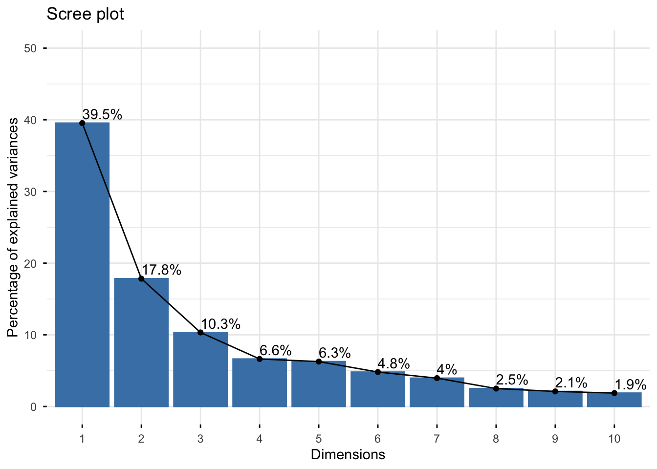
Questions: 1. What is the total inertia? What does it represent? 2. How much variance is explained by the first principal component? 3. How many components would you retain based on: - Kaiser’s criterion (eigenvalue > 1)? - The scree plot (elbow method)? - Cumulative variance > 80%?
11.2.5 Exercise 1.5: Analyze Variables
# Variable information
res.pca.wine$var
#> $coord
#>                        Dim.1        Dim.2        Dim.3
#> Class           -0.926254970  0.008995743  0.001455532
#> Alcohol          0.320745006  0.765081878 -0.249423714
#> Malic           -0.523938968  0.353343308  0.106768927
#> Ash              0.005303332  0.499123855  0.752893873
#> Alcalinity      -0.527745510 -0.018353364  0.735934715
#> Magnesium        0.293243046  0.474914593  0.157519754
#> Phenols          0.845280435  0.106103229  0.176179003
#> Flavanoids       0.919283947 -0.002053931  0.181545346
#> Nonflavanoid    -0.628222111  0.042643790  0.204378005
#> Proanthocyanins  0.656597046  0.065150511  0.180252480
#> Intensity       -0.210165463  0.837179737 -0.165085135
#> Hue              0.651277342 -0.439230962  0.102553090
#> OD280            0.824731333 -0.257193550  0.199875561
#> Proline          0.634141134  0.578427201 -0.152345199
#>                       Dim.4       Dim.5
#> Class            0.11784862 -0.14774871
#> Alcohol         -0.07872296  0.23506271
#> Malic            0.45274250  0.17621343
#> Ash             -0.24061340  0.08784040
#> Alcalinity       0.06927337 -0.04367510
#> Magnesium       -0.15789854 -0.72897375
#> Phenols          0.18416119  0.13536468
#> Flavanoids       0.13942393  0.10481942
#> Nonflavanoid    -0.31562431  0.40549009
#> Proanthocyanins  0.44562282 -0.08620346
#> Intensity        0.06949662  0.04324534
#> Hue             -0.41878540  0.02822330
#> OD280            0.15113759  0.13497146
#> Proline         -0.24640695  0.07928732
#>
#> $cor
#>                        Dim.1        Dim.2        Dim.3
#> Class           -0.926254970  0.008995743  0.001455532
#> Alcohol          0.320745006  0.765081878 -0.249423714
#> Malic           -0.523938968  0.353343308  0.106768927
#> Ash              0.005303332  0.499123855  0.752893873
#> Alcalinity      -0.527745510 -0.018353364  0.735934715
#> Magnesium        0.293243046  0.474914593  0.157519754
#> Phenols          0.845280435  0.106103229  0.176179003
#> Flavanoids       0.919283947 -0.002053931  0.181545346
#> Nonflavanoid    -0.628222111  0.042643790  0.204378005
#> Proanthocyanins  0.656597046  0.065150511  0.180252480
#> Intensity       -0.210165463  0.837179737 -0.165085135
#> Hue              0.651277342 -0.439230962  0.102553090
#> OD280            0.824731333 -0.257193550  0.199875561
#> Proline          0.634141134  0.578427201 -0.152345199
#>                       Dim.4       Dim.5
#> Class            0.11784862 -0.14774871
#> Alcohol         -0.07872296  0.23506271
#> Malic            0.45274250  0.17621343
#> Ash             -0.24061340  0.08784040
#> Alcalinity       0.06927337 -0.04367510
#> Magnesium       -0.15789854 -0.72897375
#> Phenols          0.18416119  0.13536468
#> Flavanoids       0.13942393  0.10481942
#> Nonflavanoid    -0.31562431  0.40549009
#> Proanthocyanins  0.44562282 -0.08620346
#> Intensity        0.06949662  0.04324534
#> Hue             -0.41878540  0.02822330
#> OD280            0.15113759  0.13497146
#> Proline         -0.24640695  0.07928732
#>
#> $cos2
#>                         Dim.1          Dim.2          Dim.3
#> Class           0.85794827007 0.000080923388 0.000002118574
#> Alcohol         0.10287735901 0.585350279703 0.062212189281
#> Malic           0.27451204195 0.124851492966 0.011399603795
#> Ash             0.00002812534 0.249124623086 0.566849183514
#> Alcalinity      0.27851532381 0.000336845964 0.541599904721
#> Magnesium       0.08599148401 0.225543870497 0.024812473034
#> Phenols         0.71449901365 0.011257895239 0.031039041140
#> Flavanoids      0.84508297442 0.000004218634 0.032958712515
#> Nonflavanoid    0.39466302098 0.001818492852 0.041770369089
#> Proanthocyanins 0.43111968072 0.004244589103 0.032490956713
#> Intensity       0.04416952174 0.700869911687 0.027253101873
#> Hue             0.42416217601 0.192923838123 0.010517136189
#> OD280           0.68018177233 0.066148521925 0.039950240054
#> Proline         0.40213497811 0.334578026779 0.023209059516
#>                       Dim.4        Dim.5
#> Class           0.013888297 0.0218296819
#> Alcohol         0.006197305 0.0552544793
#> Malic           0.204975773 0.0310511715
#> Ash             0.057894807 0.0077159357
#> Alcalinity      0.004798799 0.0019075141
#> Magnesium       0.024931950 0.5314027288
#> Phenols         0.033915344 0.0183235956
#> Flavanoids      0.019439032 0.0109871115
#> Nonflavanoid    0.099618708 0.1644222095
#> Proanthocyanins 0.198579697 0.0074310367
#> Intensity       0.004829780 0.0018701596
#> Hue             0.175381215 0.0007965545
#> OD280           0.022842570 0.0182172962
#> Proline         0.060716384 0.0062864784
#>
#> $contrib
#>                         Dim.1         Dim.2         Dim.3
#> Class           15.4979403483  0.0032406512  0.0001465063
#> Alcohol          1.8583721522 23.4408882298  4.3021737218
#> Malic            4.9587736225  4.9997924207  0.7883194025
#> Ash              0.0005080548  9.9764237714 39.1994509394
#> Alcalinity       5.0310887324  0.0134893053 37.4533818012
#> Magnesium        1.5533464384  9.0321109301  1.7158626098
#> Phenols         12.9066792006  0.4508327290  2.1464498949
#> Flavanoids      15.2655422056  0.0001689391  2.2792013675
#> Nonflavanoid     7.1291756977  0.0728232123  2.8885558654
#> Proanthocyanins  7.7877272185  0.1699784594  2.2468545438
#> Intensity        0.7978763254 28.0669777279  1.8846399728
#> Hue              7.6620471550  7.7258118482  0.7272939188
#> OD280           12.2867740414  2.6489781636  2.7626880669
#> Proline          7.2641488073 13.3984836120  1.6049813889
#>                      Dim.4       Dim.5
#> Class            1.4965681  2.48772450
#> Alcohol          0.6678061  6.29683580
#> Malic           22.0876767  3.53861136
#> Ash              6.2385996  0.87931297
#> Alcalinity       0.5171066  0.21738153
#> Magnesium        2.6866046 60.55899480
#> Phenols          3.6546326  2.08816867
#> Flavanoids       2.0947014  1.25209826
#> Nonflavanoid    10.7346628 18.73766015
#> Proanthocyanins 21.3984515  0.84684570
#> Intensity        0.5204450  0.21312459
#> Hue             18.8986411  0.09077586
#> OD280            2.4614582  2.07605472
#> Proline          6.5426457  0.71641110

# Correlations between variables and components
res.pca.wine$var$cor
#>                        Dim.1        Dim.2        Dim.3
#> Class           -0.926254970  0.008995743  0.001455532
#> Alcohol          0.320745006  0.765081878 -0.249423714
#> Malic           -0.523938968  0.353343308  0.106768927
#> Ash              0.005303332  0.499123855  0.752893873
#> Alcalinity      -0.527745510 -0.018353364  0.735934715
#> Magnesium        0.293243046  0.474914593  0.157519754
#> Phenols          0.845280435  0.106103229  0.176179003
#> Flavanoids       0.919283947 -0.002053931  0.181545346
#> Nonflavanoid    -0.628222111  0.042643790  0.204378005
#> Proanthocyanins  0.656597046  0.065150511  0.180252480
#> Intensity       -0.210165463  0.837179737 -0.165085135
#> Hue              0.651277342 -0.439230962  0.102553090
#> OD280            0.824731333 -0.257193550  0.199875561
#> Proline          0.634141134  0.578427201 -0.152345199
#>                       Dim.4       Dim.5
#> Class            0.11784862 -0.14774871
#> Alcohol         -0.07872296  0.23506271
#> Malic            0.45274250  0.17621343
#> Ash             -0.24061340  0.08784040
#> Alcalinity       0.06927337 -0.04367510
#> Magnesium       -0.15789854 -0.72897375
#> Phenols          0.18416119  0.13536468
#> Flavanoids       0.13942393  0.10481942
#> Nonflavanoid    -0.31562431  0.40549009
#> Proanthocyanins  0.44562282 -0.08620346
#> Intensity        0.06949662  0.04324534
#> Hue             -0.41878540  0.02822330
#> OD280            0.15113759  0.13497146
#> Proline         -0.24640695  0.07928732

# Coordinates of variables
res.pca.wine$var$coord
#>                        Dim.1        Dim.2        Dim.3
#> Class           -0.926254970  0.008995743  0.001455532
#> Alcohol          0.320745006  0.765081878 -0.249423714
#> Malic           -0.523938968  0.353343308  0.106768927
#> Ash              0.005303332  0.499123855  0.752893873
#> Alcalinity      -0.527745510 -0.018353364  0.735934715
#> Magnesium        0.293243046  0.474914593  0.157519754
#> Phenols          0.845280435  0.106103229  0.176179003
#> Flavanoids       0.919283947 -0.002053931  0.181545346
#> Nonflavanoid    -0.628222111  0.042643790  0.204378005
#> Proanthocyanins  0.656597046  0.065150511  0.180252480
#> Intensity       -0.210165463  0.837179737 -0.165085135
#> Hue              0.651277342 -0.439230962  0.102553090
#> OD280            0.824731333 -0.257193550  0.199875561
#> Proline          0.634141134  0.578427201 -0.152345199
#>                       Dim.4       Dim.5
#> Class            0.11784862 -0.14774871
#> Alcohol         -0.07872296  0.23506271
#> Malic            0.45274250  0.17621343
#> Ash             -0.24061340  0.08784040
#> Alcalinity       0.06927337 -0.04367510
#> Magnesium       -0.15789854 -0.72897375
#> Phenols          0.18416119  0.13536468
#> Flavanoids       0.13942393  0.10481942
#> Nonflavanoid    -0.31562431  0.40549009
#> Proanthocyanins  0.44562282 -0.08620346
#> Intensity        0.06949662  0.04324534
#> Hue             -0.41878540  0.02822330
#> OD280            0.15113759  0.13497146
#> Proline         -0.24640695  0.07928732

# Quality of representation (cos²)
res.pca.wine$var$cos2
#>                         Dim.1          Dim.2          Dim.3
#> Class           0.85794827007 0.000080923388 0.000002118574
#> Alcohol         0.10287735901 0.585350279703 0.062212189281
#> Malic           0.27451204195 0.124851492966 0.011399603795
#> Ash             0.00002812534 0.249124623086 0.566849183514
#> Alcalinity      0.27851532381 0.000336845964 0.541599904721
#> Magnesium       0.08599148401 0.225543870497 0.024812473034
#> Phenols         0.71449901365 0.011257895239 0.031039041140
#> Flavanoids      0.84508297442 0.000004218634 0.032958712515
#> Nonflavanoid    0.39466302098 0.001818492852 0.041770369089
#> Proanthocyanins 0.43111968072 0.004244589103 0.032490956713
#> Intensity       0.04416952174 0.700869911687 0.027253101873
#> Hue             0.42416217601 0.192923838123 0.010517136189
#> OD280           0.68018177233 0.066148521925 0.039950240054
#> Proline         0.40213497811 0.334578026779 0.023209059516
#>                       Dim.4        Dim.5
#> Class           0.013888297 0.0218296819
#> Alcohol         0.006197305 0.0552544793
#> Malic           0.204975773 0.0310511715
#> Ash             0.057894807 0.0077159357
#> Alcalinity      0.004798799 0.0019075141
#> Magnesium       0.024931950 0.5314027288
#> Phenols         0.033915344 0.0183235956
#> Flavanoids      0.019439032 0.0109871115
#> Nonflavanoid    0.099618708 0.1644222095
#> Proanthocyanins 0.198579697 0.0074310367
#> Intensity       0.004829780 0.0018701596
#> Hue             0.175381215 0.0007965545
#> OD280           0.022842570 0.0182172962
#> Proline         0.060716384 0.0062864784

# Contributions
res.pca.wine$var$contrib
#>                         Dim.1         Dim.2         Dim.3
#> Class           15.4979403483  0.0032406512  0.0001465063
#> Alcohol          1.8583721522 23.4408882298  4.3021737218
#> Malic            4.9587736225  4.9997924207  0.7883194025
#> Ash              0.0005080548  9.9764237714 39.1994509394
#> Alcalinity       5.0310887324  0.0134893053 37.4533818012
#> Magnesium        1.5533464384  9.0321109301  1.7158626098
#> Phenols         12.9066792006  0.4508327290  2.1464498949
#> Flavanoids      15.2655422056  0.0001689391  2.2792013675
#> Nonflavanoid     7.1291756977  0.0728232123  2.8885558654
#> Proanthocyanins  7.7877272185  0.1699784594  2.2468545438
#> Intensity        0.7978763254 28.0669777279  1.8846399728
#> Hue              7.6620471550  7.7258118482  0.7272939188
#> OD280           12.2867740414  2.6489781636  2.7626880669
#> Proline          7.2641488073 13.3984836120  1.6049813889
#>                      Dim.4       Dim.5
#> Class            1.4965681  2.48772450
#> Alcohol          0.6678061  6.29683580
#> Malic           22.0876767  3.53861136
#> Ash              6.2385996  0.87931297
#> Alcalinity       0.5171066  0.21738153
#> Magnesium        2.6866046 60.55899480
#> Phenols          3.6546326  2.08816867
#> Flavanoids       2.0947014  1.25209826
#> Nonflavanoid    10.7346628 18.73766015
#> Proanthocyanins 21.3984515  0.84684570
#> Intensity        0.5204450  0.21312459
#> Hue             18.8986411  0.09077586
#> OD280            2.4614582  2.07605472
#> Proline          6.5426457  0.71641110
Questions: 1. Which variables are most correlated with the first principal component? 2. Which variables contribute most to the first dimension? 3. Which variables are well represented in the first two dimensions (cos² > 0.5)?
11.2.6 Exercise 1.6: Visualize Variables
# Basic variable plot
fviz_pca_var(res.pca.wine, col.var = "black")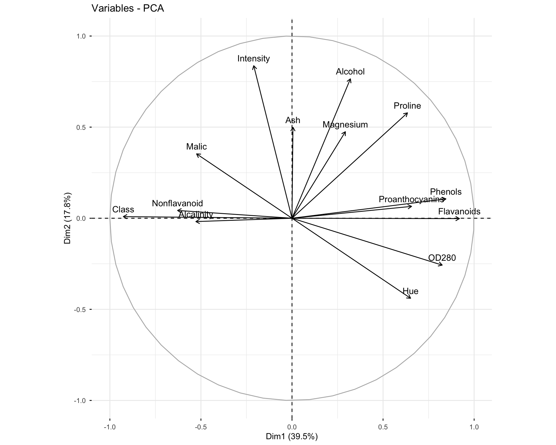
# Variables colored by quality of representation
fviz_pca_var(res.pca.wine, col.var = "cos2",
             gradient.cols = c("#00AFBB", "#E7B800", "#FC4E07"),
             repel = TRUE)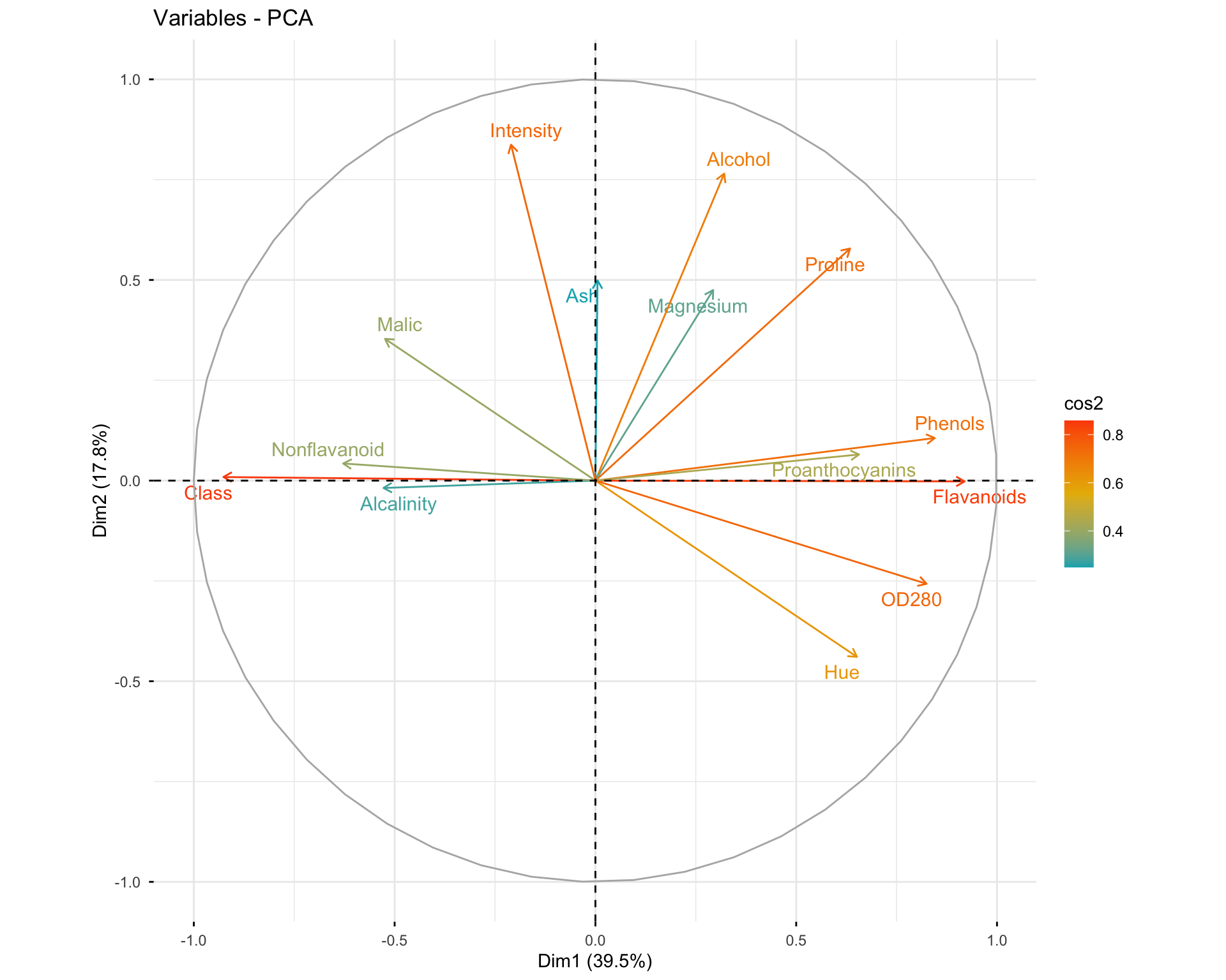
# Variables colored by contributions
fviz_pca_var(res.pca.wine, col.var = "contrib",
             gradient.cols = c("#00AFBB", "#E7B800", "#FC4E07"),
             repel = TRUE)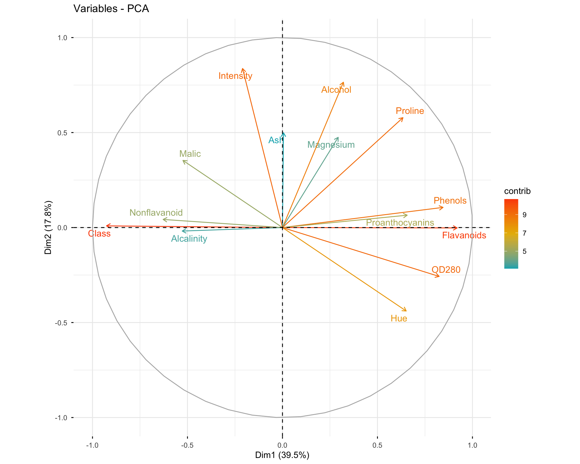
Questions: 1. What do the arrows represent in the variable plot? 2. What does the length of an arrow indicate? 3. What does the angle between two arrows tell you about the correlation between variables?
11.2.7 Exercise 1.7: Analyze Individuals
# Individual information
res.pca.wine$ind
#> $coord
#>            Dim.1       Dim.2        Dim.3           Dim.4
#> 1    3.522918024  1.45311867 -0.164772369 -0.013926256309
#> 2    2.528847526 -0.32999903 -2.026697043 -0.416667812490
#> 3    2.785007148  1.03697906  0.983264785  0.664373920551
#> 4    3.922570237  2.76829806 -0.174937730  0.565415182346
#> 5    1.407474906  0.86779758  2.025818285 -0.441145568025
#> 6    3.288108428  2.13017591 -0.629015963 -0.605056582516
#> 7    2.750561100  1.17918568 -0.977347561 -0.352717758232
#> 8    2.392844659  1.61125983  0.145704264 -1.245777972022
#> 9    2.795235652  0.92319068 -1.770949667 -0.156056378845
#> 10   3.005576356  0.79634006 -0.983728735  0.270841737770
#> 11   3.678663918  1.31249164 -0.421876929  0.002039556136
#> 12   2.109617169  0.61292670 -1.191610706 -1.098132793011
#> 13   2.438433322  0.67850437 -0.865549463 -0.657896417360
#> 14   3.673459480  1.14011683 -1.203831869 -0.229927298528
#> 15   4.441551027  2.11031094 -1.262480181  0.204510749383
#> 16   2.608885294  1.66635097  0.217554034 -1.518471831413
#> 17   2.475402186  2.33086927  0.831571622 -0.897632785058
#> 18   2.226198712  1.63356578  0.794509929 -1.150203812077
#> 19   3.742235824  2.52836126 -0.484902514 -1.054210285615
#> 20   2.394389854  1.06458639 -0.164684915  0.566957738763
#> 21   3.336546971  0.79604355 -0.363831481  0.245993076967
#> 22   1.481371313  0.24014421  0.936244720  0.899853157412
#> 23   2.828047560 -0.08683042 -0.311959826 -0.206442226612
#> 24   2.007694727 -0.51560048  0.143263270 -0.577870366709
#> 25   2.114606195 -0.31588971  0.889721704 -0.331014695515
#> 26   1.397496000  0.93820161  3.819815976 -1.347993684779
#> 27   2.133470441  0.68715566 -0.087451244 -0.574878222594
#> 28   1.629698090 -0.09119739 -1.387811890 -0.674076101573
#> 29   2.507562173  0.69274094  1.394115208 -0.986467655274
#> 30   2.559467329  0.19550527 -1.092667881  0.132383587928
#> 31   2.772412896  1.24633503  1.386231386 -0.446487436226
#> 32   2.935118156  1.47826152 -0.331854355 -0.321188592884
#> 33   1.991220330  0.05320941 -0.167859145 -0.933901583246
#> 34   2.245672360  1.63458672  1.171302514 -2.355848725794
#> 35   1.786966008  0.69744752  0.478942465 -1.100686266672
#> 36   2.227614790  0.17933442  0.450741651  0.202344151093
#> 37   1.768001103  0.65785833  0.457489360 -1.386791557466
#> 38   1.523158040  0.11219285 -0.040133237 -1.099178499752
#> 39   1.872350633 -0.76934180 -1.426833311 -0.845227013710
#> 40   2.797090511  1.80889925 -0.342619705  1.343216049323
#> 41   2.840916446  0.78623506 -0.117743376  0.601278338096
#> 42   1.105551874  0.16595498 -0.784551968  0.978955102017
#> 43   3.306878987  1.16405408 -0.312155721  0.454650276704
#> 44   0.904775408  0.32617794 -0.202549074  1.250427540974
#> 45   2.396828265 -0.06681908 -0.655418561  0.840769963831
#> 46   1.537782793  1.77514833  0.027663137  0.446173159986
#> 47   2.991183721  1.19769630 -0.539468583  1.167086205149
#> 48   3.059304804  0.65390980 -1.154706807  0.997424851524
#> 49   2.318745488  1.25024762 -0.057311669  0.139415862876
#> 50   2.959443594  1.75860262 -0.642687006 -0.145556586359
#> 51   3.412171503  0.17693942 -1.972247667  1.205357522972
#> 52   3.116351685  0.75208225  0.004972309 -0.366222301627
#> 53   3.700183236  1.62315920 -0.519870174  0.039826980905
#> 54   2.537518381  1.87849370  0.339130859 -1.330818167782
#> 55   2.444783767  1.02074113 -0.957532313 -0.058927476567
#> 56   2.722800840  1.33527318  0.514232404  0.507816922262
#> 57   2.985299567  1.44369364 -0.611767379  0.332163476572
#> 58   2.488120327  1.21550134  0.261472497 -0.680110072401
#> 59   3.351275971  1.74066764 -0.284691036  0.315764384011
#> 60  -0.874923506 -3.07776508 -4.585651475 -0.959203519966
#> 61  -1.414697443 -1.39006863 -0.876591591 -3.099592771276
#> 62  -1.713906251 -0.83888496 -1.607134490 -1.521529500895
#> 63   0.012264892 -1.26275166 -1.784675940 -1.253874698452
#> 64   1.833060109 -1.91331687 -0.005299173  0.897387099618
#> 65  -0.574586722 -1.91126123  0.678573508 -2.111807610124
#> 66   0.791438409 -0.75874544  0.574170996 -0.555872993625
#> 67   2.020004353 -1.87204562 -2.029678832  1.428241960032
#> 68   0.143252297 -2.42572107 -1.069518855  0.040165191987
#> 69  -0.751534609 -0.22526038 -0.708228071 -2.591053825474
#> 70   1.740331083 -1.39112032 -1.235538486  0.039068672956
#> 71  -1.471439977 -0.89718602 -0.628427567 -0.988141665576
#> 72   1.491915521 -0.94790641  1.953781747  0.098574608933
#> 73  -0.693995613 -1.06683281  0.079855830 -0.155179627430
#> 74   2.299416093  0.27432413  3.376821913 -0.298256092532
#> 75   1.634117569 -1.27732363  0.460261134  0.558016383438
#> 76  -0.829023350 -2.44776670 -1.563736486 -0.663736199569
#> 77   0.300409802 -2.15108078 -2.448756951 -0.004978565189
#> 78  -1.361197617 -1.39035146 -0.228301605 -0.565960852175
#> 79   1.096056532 -0.76270658 -1.182313542 -0.113826485462
#> 80   0.319163039 -1.02471772  1.794789911  0.893377696157
#> 81   0.671218081 -3.37053621 -0.356728629 -0.291128734738
#> 82   0.924081966 -1.44508906 -0.362171117  0.290344185286
#> 83  -0.467533679 -2.38381074  1.335086204 -1.243193954847
#> 84  -2.352456493 -0.10009045  0.472208786  0.303199333284
#> 85   0.718223070 -1.46801633  0.611456423  0.887862534258
#> 86   0.698267141 -2.02225187 -0.254076524 -0.654741954248
#> 87  -0.764614511 -2.23757347  0.772209534 -1.053428568007
#> 88  -0.528298761 -2.37574381  2.306992109 -1.131988339156
#> 89  -1.037882647 -1.80784436  0.958255703 -0.556799710056
#> 90  -0.521454457 -2.66034115  0.848508573 -0.333890062869
#> 91  -1.253385943 -2.12476709 -0.048831395 -0.716748514566
#> 92  -1.460737746 -1.85970760  0.779915804 -0.751206591727
#> 93  -1.791269332 -1.56916686 -0.090891613 -0.848499440696
#> 94   0.653267701 -2.30832502  0.115578330  1.291404235650
#> 95   0.836110472 -2.21749637  0.143675225  0.598449579199
#> 96   2.260607925  0.18420714  0.791778051  0.107223958898
#> 97  -0.555475848 -0.37017528  1.309299852 -0.500762885462
#> 98   0.914966608 -2.55962010 -1.085374266  0.320159081868
#> 99   2.020956911 -1.42012011 -0.228006470  1.065188559812
#> 100  1.265369320 -2.15846340  0.750084481  1.101680411018
#> 101  0.701408366 -2.37224214 -1.567252507  0.162531212051
#> 102 -0.530878379 -2.29536665 -1.499153846 -0.245322464454
#> 103 -0.176180924 -1.16467140  1.003815322  0.666258772024
#> 104 -0.642757821 -2.68222523 -0.764965455  0.489624432343
#> 105  0.337684658 -2.09634737 -0.471464417  0.373210178737
#> 106 -1.637243635 -1.72628691  0.945496724 -0.112048754597
#> 107 -0.358792560 -2.17077498 -0.481497360  0.267832752044
#> 108 -1.513137651 -1.36332666  0.286015956 -0.222574288009
#> 109  0.030085767 -2.30440977 -0.462843182  1.015552058557
#> 110  1.409384663 -1.45302142  1.781306223  0.808846799143
#> 111  1.218241291 -1.40802222  0.142033338  3.980861651997
#> 112 -0.288339800 -1.93112525  0.078799001  0.921339147101
#> 113 -1.196150183 -0.77050190  1.997955246 -1.955769508799
#> 114 -0.451648526 -2.27099330  1.061175579 -0.824900104449
#> 115 -0.471872764 -1.94128941  1.323493045 -0.271742861692
#> 116  0.423335647 -3.86908307  1.344504539 -0.981581626116
#> 117 -0.264386608 -2.82185500 -0.302410448  0.530207298139
#> 118 -0.137480398 -1.92843774  0.690521366  0.000003777304
#> 119 -2.250493332 -1.26924005 -1.904889359  0.521247520695
#> 120 -0.530762515 -2.22434284 -0.356373349  1.281102040255
#> 121  0.641269477 -1.40417218  1.126394008  1.314097940594
#> 122  1.184313109  0.26109499  5.346739245  0.424255737293
#> 123 -1.106989025 -0.66940397  3.009473590  1.049444710996
#> 124 -0.458685486 -0.61969330  0.483528490  3.340328691512
#> 125  0.846080621 -1.43888467  1.482895360  3.812233406981
#> 126 -0.116562375 -2.10977446  0.435006063  0.940511428521
#> 127 -0.007104989 -1.26534660  0.688125194  1.216000486737
#> 128 -1.495350135 -1.21563545  3.360056786 -0.405213961113
#> 129 -0.478624084 -1.94018917  1.296591584  0.671430006317
#> 130 -1.664175709 -1.15908430  0.781458268  1.124477941226
#> 131 -1.778943684  0.17228098 -1.178839590 -0.811122551453
#> 132 -2.741937196  0.37086548 -0.723644039  0.007978757817
#> 133 -3.254310403  0.25758026 -0.167772216 -0.136230480148
#> 134 -2.530388335  0.36600160 -0.452791227  0.446222088451
#> 135 -2.713045332 -0.46385329 -1.101657507 -0.975228943525
#> 136 -3.349016441  0.34557115 -1.099962707 -0.872689425080
#> 137 -4.117202383  0.14198595  0.220163264 -0.262019929513
#> 138 -4.144188872  0.64725279  1.710611538  0.243564793427
#> 139 -3.365967328  0.34042878 -1.027933346 -0.378232282634
#> 140 -2.712726623  0.28748293  1.241490172 -0.819120395687
#> 141 -3.071680894  0.27982578  0.608754978 -1.036780148849
#> 142 -2.626166752  0.36826427 -0.972006044 -0.463214345208
#> 143 -3.260445573  0.48108190  0.945777489 -1.224089680201
#> 144 -2.704101752  0.47749459 -0.253449336  0.411957890958
#> 145 -2.590861219  1.15752557 -1.244609569  0.708157077476
#> 146 -2.954020852  0.55788774 -0.856127602  0.377083744097
#> 147 -4.459981559  0.63554443 -1.459954363  0.796730909228
#> 148 -3.829287610  1.26243010 -0.111881921  0.787547685624
#> 149 -3.133679945  1.56472907 -0.472756720  0.573132232904
#> 150 -3.234739627  2.03537390 -0.495858512  0.795513733990
#> 151 -2.712586051  2.35391168  0.438405959  0.525586720303
#> 152 -2.930956654  2.04205722 -0.311521488  0.900358039242
#> 153 -2.250596974  1.52801594  1.363790357  0.375871613090
#> 154 -3.097551711  2.13354943 -0.964742195  0.617163741854
#> 155 -3.077061476  0.40481612 -1.190315380 -0.421982081968
#> 156 -3.856200626  1.79216205 -0.095077401  1.004947457457
#> 157 -3.208428815  1.91892539 -0.782669567  1.148803410016
#> 158 -3.658532777  1.30261252  1.601038597 -0.624064644708
#> 159 -1.553028400  3.51920834  1.161564432  1.008796841684
#> 160 -2.058323722  2.40765703  0.549547794  0.751773271073
#> 161 -3.438586574  0.73065802 -0.091486383  0.842493585950
#> 162 -2.584536514  1.17128882 -0.101889526 -1.204679422191
#> 163 -3.144502558  0.54902947  0.803394762 -0.964981063827
#> 164 -2.925312657  0.69267412 -0.885201944 -0.131319821967
#> 165 -3.261861712  1.54861450 -0.983862644 -0.039040516391
#> 166 -3.777633103  0.87233703 -0.467215210  0.314181929664
#> 167 -2.774690234  2.58869214  0.428315610 -0.008883452551
#> 168 -3.242652681  1.26788019 -1.213773958  0.240500463334
#> 169 -2.563777659  2.07491544  0.764034442 -0.207218518733
#> 170 -2.748775899  2.58514396  1.418234806  0.808481977825
#> 171 -3.491213954 -0.25942579 -0.847744623 -0.124978958578
#> 172 -3.929162637  0.83744474 -1.340388581 -0.231244399843
#> 173 -2.815329157  2.18938428 -0.918984300 -0.080588573166
#> 174 -3.628044277  2.20668032 -0.343744501  0.752446911509
#> 175 -2.942765014  1.75229589  0.207438633  0.399123143134
#> 176 -3.027298525  2.75606589 -0.940832565  0.606660438947
#> 177 -2.755240485  2.29379266 -0.550497752 -0.392512052691
#> 178 -3.496390966  2.76068615  1.013070513  0.350429769737
#>            Dim.5
#> 1   -0.737323391
#> 2    0.283643924
#> 3    0.386990929
#> 4    0.323943110
#> 5   -0.227517055
#> 6    0.410148340
#> 7    1.024613744
#> 8   -0.206295854
#> 9    0.858541111
#> 10   0.471657012
#> 11   0.259699455
#> 12   0.558828290
#> 13   1.088276889
#> 14   1.822655142
#> 15   0.844212099
#> 16   0.100892900
#> 17  -0.210265249
#> 18   0.131484326
#> 19   0.723193967
#> 20  -0.537541332
#> 21  -0.968868318
#> 22   0.209048350
#> 23   0.487810262
#> 24   0.377283258
#> 25   0.624309150
#> 26  -0.341365748
#> 27   1.131067011
#> 28   0.375394077
#> 29   0.632318904
#> 30   0.574806483
#> 31   0.410905993
#> 32  -0.057358996
#> 33   0.488402862
#> 34  -0.349402029
#> 35  -0.222978993
#> 36   0.272882427
#> 37   0.001395361
#> 38   0.205623377
#> 39   0.066339885
#> 40  -0.742345225
#> 41  -0.324826083
#> 42   0.971115608
#> 43   0.449752734
#> 44   0.385982834
#> 45  -0.249037726
#> 46   0.537857656
#> 47   0.920943379
#> 48   0.201025005
#> 49   0.404392512
#> 50   0.341456879
#> 51   0.104318822
#> 52   0.636970440
#> 53   0.492816782
#> 54   0.277707075
#> 55  -0.837065241
#> 56  -0.860204322
#> 57  -0.394865003
#> 58   0.568334604
#> 59  -0.113148447
#> 60  -0.628510026
#> 61   0.277964474
#> 62  -0.045816489
#> 63   0.062319939
#> 64  -0.037583818
#> 65  -0.477048892
#> 66  -0.229480101
#> 67   0.717201861
#> 68   0.477479733
#> 69  -0.020857116
#> 70  -4.449208881
#> 71  -1.114792520
#> 72   0.602798498
#> 73   0.204118007
#> 74  -2.342893243
#> 75  -1.102485083
#> 76  -0.845959276
#> 77  -0.255926169
#> 78  -0.979319399
#> 79  -2.927608020
#> 80   0.418980632
#> 81  -0.082937999
#> 82   0.267399853
#> 83   0.697470861
#> 84   1.463920234
#> 85  -0.855763132
#> 86  -0.533834919
#> 87   0.013784273
#> 88   0.209184145
#> 89   0.685214943
#> 90   1.279858920
#> 91   0.783467330
#> 92   0.374992140
#> 93   1.040657338
#> 94   0.053214661
#> 95  -0.895966897
#> 96  -4.078060769
#> 97  -3.393171649
#> 98   0.098100704
#> 99   0.144774597
#> 100  0.822637255
#> 101 -0.648601021
#> 102 -0.350899187
#> 103 -0.045402401
#> 104 -0.025544183
#> 105  0.372891825
#> 106  1.175100971
#> 107  0.548536786
#> 108  0.599287649
#> 109 -0.206093088
#> 110 -0.315624213
#> 111 -1.396107944
#> 112  0.049819834
#> 113  0.407657677
#> 114 -0.007586959
#> 115  0.796580957
#> 116  0.492734780
#> 117 -0.233233266
#> 118 -1.093626855
#> 119  0.946268623
#> 120  0.271573407
#> 121 -0.157209361
#> 122 -0.351421221
#> 123  0.207936048
#> 124  1.012235685
#> 125  0.465310820
#> 126  0.571575372
#> 127  0.551441476
#> 128  0.584910716
#> 129  0.191939831
#> 130  1.109843388
#> 131 -2.677819004
#> 132 -1.318550609
#> 133 -1.136642981
#> 134 -1.589463531
#> 135  0.624115280
#> 136  0.467430159
#> 137  0.573555564
#> 138  0.861947883
#> 139  1.060044947
#> 140  0.200126475
#> 141  0.379583579
#> 142  0.266203811
#> 143  0.411069487
#> 144  0.902940787
#> 145 -1.504851571
#> 146 -0.478943995
#> 147  0.919530173
#> 148  0.901470026
#> 149  0.355067798
#> 150 -1.241496895
#> 151 -2.186602621
#> 152 -1.779940143
#> 153 -1.906691765
#> 154  0.480674109
#> 155 -0.778515638
#> 156  0.994703553
#> 157  0.861865624
#> 158  0.489125606
#> 159  0.615135593
#> 160  0.742014747
#> 161  0.637352140
#> 162 -0.017023996
#> 163  0.061936001
#> 164 -0.722816090
#> 165  0.289898075
#> 166  0.897780625
#> 167 -0.564900315
#> 168  0.291597025
#> 169 -0.563390938
#> 170 -0.865848227
#> 171 -0.548793467
#> 172  0.398204711
#> 173  0.560024117
#> 174  1.003241669
#> 175 -0.154695420
#> 176 -1.128844821
#> 177 -1.066773471
#> 178  1.004719829
#>
#> $cos2
#>              Dim.1        Dim.2          Dim.3
#> 1   0.710132531677 0.1208193508 0.001553470838
#> 2   0.494663065848 0.0084234406 0.317718031367
#> 3   0.620093143078 0.0859694752 0.077293909029
#> 4   0.614376885232 0.3059983651 0.001221969551
#> 5   0.230576205622 0.0876536563 0.477676790684
#> 6   0.634513636960 0.2663051950 0.023220524968
#> 7   0.585355713819 0.1075825081 0.073905257766
#> 8   0.451539842647 0.2047378917 0.001674216386
#> 9   0.561323589111 0.0612292949 0.225314362042
#> 10  0.740835777254 0.0520072091 0.079362827272
#> 11  0.751708646894 0.0956890875 0.009886461341
#> 12  0.469958771741 0.0396706707 0.149941292604
#> 13  0.603840463055 0.0467525975 0.076082403751
#> 14  0.531596271531 0.0512070940 0.057090400707
#> 15  0.657953445043 0.1485315637 0.053158778335
#> 16  0.516467915988 0.2107008727 0.003591432085
#> 17  0.447818728892 0.3970512305 0.050537067015
#> 18  0.464208736268 0.2499532040 0.059126764320
#> 19  0.564779875675 0.2578072718 0.009482563979
#> 20  0.517235782902 0.1022493727 0.002446845099
#> 21  0.724910449533 0.0412632594 0.008619665678
#> 22  0.286983680336 0.0075417754 0.114632589635
#> 23  0.785535019758 0.0007405186 0.009558493980
#> 24  0.581256740793 0.0383353352 0.002959663704
#> 25  0.569311415845 0.0127046249 0.100785780270
#> 26  0.095458191292 0.0430233674 0.713176355361
#> 27  0.528168949315 0.0547910794 0.000887424865
#> 28  0.359024138746 0.0011242791 0.260357770324
#> 29  0.578527026880 0.0441531756 0.178820606139
#> 30  0.699635016498 0.0040821532 0.127511311276
#> 31  0.539192658813 0.1089676921 0.134803014865
#> 32  0.636187594580 0.1613751146 0.008132593430
#> 33  0.607191864575 0.0004335750 0.004314965428
#> 34  0.298279656321 0.1580326335 0.081146351387
#> 35  0.514170607507 0.0783245178 0.036935276385
#> 36  0.788021067083 0.0051072246 0.032263614871
#> 37  0.371655276973 0.0514564704 0.024884976584
#> 38  0.454579477222 0.0024663248 0.000315593658
#> 39  0.467192411295 0.0788787590 0.271311308255
#> 40  0.386477053732 0.1616364970 0.005798762854
#> 41  0.707557771654 0.0541938238 0.001215396415
#> 42  0.168635121521 0.0037998840 0.084924541686
#> 43  0.700775197479 0.0868337254 0.006244313726
#> 44  0.140506822341 0.0182610194 0.007041681243
#> 45  0.704461286640 0.0005475002 0.052676967898
#> 46  0.217645225589 0.2900203338 0.000070430702
#> 47  0.608529116944 0.0975637768 0.019793723612
#> 48  0.732371557395 0.0334596709 0.104334856754
#> 49  0.641159312892 0.1864025556 0.000391693089
#> 50  0.607553089322 0.2145356803 0.028652540704
#> 51  0.555176308935 0.0014928577 0.185477880299
#> 52  0.717872594698 0.0418104772 0.000001827556
#> 53  0.700756747290 0.1348475500 0.013832816934
#> 54  0.514802881215 0.2821253190 0.009195115640
#> 55  0.617075222875 0.1075693226 0.094659472382
#> 56  0.646662522232 0.1555199804 0.023065603357
#> 57  0.695171719811 0.1625797104 0.029193683238
#> 58  0.624724184088 0.1490927217 0.006899181800
#> 59  0.688459710817 0.1857333337 0.004968276196
#> 60  0.022301601510 0.2759731423 0.612629590060
#> 61  0.116450526529 0.1124311892 0.044710437512
#> 62  0.252826117182 0.0605693106 0.222306546634
#> 63  0.000016487434 0.1747678501 0.349095608259
#> 64  0.261885498698 0.2853197528 0.000002188640
#> 65  0.028757949734 0.3181902362 0.040108881360
#> 66  0.130082854120 0.1195578227 0.068464952590
#> 67  0.227036608087 0.1949952951 0.229216524663
#> 68  0.001885878850 0.5407447631 0.105120518171
#> 69  0.048322487508 0.0043413116 0.042913860462
#> 70  0.098160217261 0.0627192916 0.049474830286
#> 71  0.251516992879 0.0935076679 0.045876754296
#> 72  0.143530978068 0.0579412823 0.246155347915
#> 73  0.071516166218 0.1689987538 0.000946899804
#> 74  0.182421941045 0.0025963901 0.393421648760
#> 75  0.240386558136 0.1468741871 0.019070065568
#> 76  0.057438402581 0.5007360637 0.204360033962
#> 77  0.006849338315 0.3511833025 0.455105185824
#> 78  0.227652344459 0.2375083915 0.006403946518
#> 79  0.065019168743 0.0314840425 0.075655556674
#> 80  0.012086668797 0.1245919350 0.382215835841
#> 81  0.032822654417 0.8276455797 0.009270909373
#> 82  0.196256369278 0.4799455805 0.030146048544
#> 83  0.018804988117 0.4888670943 0.153343679041
#> 84  0.521852403472 0.0009446910 0.021026772401
#> 85  0.051042940992 0.2132449531 0.036995424146
#> 86  0.075691727721 0.6348566853 0.010021535889
#> 87  0.065385446574 0.5599517787 0.066690863535
#> 88  0.019066663201 0.3855802002 0.363586483486
#> 89  0.149415225348 0.4533362307 0.127368248790
#> 90  0.023048282860 0.5999022225 0.061026473680
#> 91  0.173081180783 0.4973966695 0.000262711129
#> 92  0.243344826109 0.3944272802 0.069370217335
#> 93  0.306876545938 0.2354941751 0.000790113604
#> 94  0.047889004888 0.5979258908 0.001499016010
#> 95  0.066075041640 0.4647677173 0.001951074668
#> 96  0.160702341273 0.0010670496 0.019714175985
#> 97  0.017763359350 0.0078887750 0.098689961283
#> 98  0.085195212903 0.6667387984 0.119884695326
#> 99  0.336545139630 0.1661802363 0.004283744464
#> 100 0.099154041358 0.2885128730 0.034841446709
#> 101 0.043867623765 0.5017879877 0.219018183505
#> 102 0.030215923780 0.5648718503 0.240956255847
#> 103 0.006139976749 0.2683216900 0.199322625247
#> 104 0.042368428175 0.7377990645 0.060011054593
#> 105 0.016586670727 0.6392387026 0.032332136644
#> 106 0.211992248617 0.2356781463 0.070699023808
#> 107 0.019112465248 0.6996155668 0.034420539338
#> 108 0.321546222032 0.2610275750 0.011488598688
#> 109 0.000102423659 0.6008935225 0.024240738544
#> 110 0.172632171269 0.1834875845 0.275765429459
#> 111 0.054931779675 0.0733797209 0.000746685346
#> 112 0.012295188821 0.5515017626 0.000918263749
#> 113 0.102850475756 0.0426758632 0.286950109478
#> 114 0.020991536670 0.5307313509 0.115882413417
#> 115 0.025716380349 0.4352518150 0.202303476470
#> 116 0.007281768669 0.6082516655 0.073449990658
#> 117 0.007061562801 0.8044356457 0.009238798641
#> 118 0.002891609318 0.5689437086 0.072947816510
#> 119 0.372542355956 0.1184971033 0.266906842473
#> 120 0.030811372097 0.5411454420 0.013890599477
#> 121 0.050964078673 0.2443564280 0.157240241830
#> 122 0.036873530210 0.0017921680 0.751553072276
#> 123 0.085528334000 0.0312751897 0.632127166456
#> 124 0.012280323386 0.0224147249 0.013646583713
#> 125 0.034442591681 0.0996148982 0.105801869011
#> 126 0.001837000014 0.6018169937 0.025584857807
#> 127 0.000006625347 0.2101361756 0.062146508657
#> 128 0.130643669496 0.0863394531 0.659623039150
#> 129 0.028579918060 0.4696345451 0.209738558591
#> 130 0.290253072127 0.1408019001 0.064001484786
#> 131 0.212207889430 0.0019902692 0.093185116361
#> 132 0.598214811335 0.0109439721 0.041666990525
#> 133 0.676934917127 0.0042408619 0.001799156943
#> 134 0.463895162733 0.0097053558 0.014853934274
#> 135 0.504546699806 0.0147485237 0.083191789299
#> 136 0.713344931210 0.0075952133 0.076952182741
#> 137 0.786323507264 0.0009351635 0.002248467111
#> 138 0.690578438493 0.0168454182 0.117662135971
#> 139 0.761680827911 0.0077912256 0.071036759422
#> 140 0.645251329450 0.0072467118 0.135146069906
#> 141 0.738342305585 0.0061274672 0.028999506774
#> 142 0.610495281204 0.0120048537 0.083632608935
#> 143 0.681032565989 0.0148269563 0.057304920643
#> 144 0.564510184772 0.0176020248 0.004959159048
#> 145 0.444713990395 0.0887674363 0.102626321549
#> 146 0.678052433350 0.0241840928 0.056952548645
#> 147 0.704093072627 0.0142973577 0.075447092114
#> 148 0.785799621696 0.0854064208 0.000670804042
#> 149 0.724345371742 0.1805987402 0.016485868606
#> 150 0.572924649990 0.2268335298 0.013462769066
#> 151 0.349576229164 0.2632419941 0.009131197642
#> 152 0.411786494939 0.1998891048 0.004651888806
#> 153 0.293178851586 0.1351428100 0.107654554609
#> 154 0.471870987819 0.2238677645 0.045772927908
#> 155 0.586236261182 0.0101464925 0.087725211116
#> 156 0.657662796061 0.1420491324 0.000399796174
#> 157 0.588094251098 0.2103673298 0.034996048657
#> 158 0.634330376237 0.0804140811 0.121480119970
#> 159 0.076303030269 0.3918076829 0.042684441211
#> 160 0.192364399326 0.2632004245 0.013712236005
#> 161 0.760254107050 0.0343263127 0.000538160432
#> 162 0.591241987377 0.1214305389 0.000918880450
#> 163 0.758165143134 0.0231127284 0.049490050917
#> 164 0.745439293148 0.0417951245 0.068257820856
#> 165 0.652473082064 0.1470679875 0.059360896592
#> 166 0.791587064578 0.0422112055 0.012108576292
#> 167 0.452106085510 0.3935248405 0.010773061693
#> 168 0.653920755042 0.0999725304 0.091622024512
#> 169 0.476170993825 0.3118911298 0.042289065914
#> 170 0.367624981840 0.3251590266 0.097863924201
#> 171 0.842712124624 0.0046532097 0.049688558793
#> 172 0.731995652083 0.0332522324 0.085186333972
#> 173 0.495867010383 0.2998823115 0.052835161978
#> 174 0.596902474236 0.2208193191 0.005358333504
#> 175 0.690828787196 0.2449481376 0.003432721280
#> 176 0.444100826745 0.3680868277 0.042893922796
#> 177 0.454626098370 0.3150965584 0.018148738368
#> 178 0.532260921975 0.3318323144 0.044685225360
#>                   Dim.4           Dim.5
#> 1   0.00001109693650833 0.0311064433257
#> 2   0.01342901319222555 0.0062231628265
#> 3   0.03528819568321861 0.0119730796585
#> 4   0.01276522111679494 0.0041901628670
#> 5   0.02265150214418492 0.0060250559009
#> 6   0.02148526328629995 0.0098725789473
#> 7   0.00962569108770850 0.0812264781382
#> 8   0.12239068373766034 0.0033562017862
#> 9   0.00174960290077589 0.0529539830093
#> 10  0.00601585831958939 0.0182439556099
#> 11  0.00000023106844788 0.0037463763085
#> 12  0.12733921823221608 0.0329768542178
#> 13  0.04395572882146736 0.1202760772866
#> 14  0.00208263178524840 0.1308700984289
#> 15  0.00139494836961541 0.0237699899155
#> 16  0.17496325832725160 0.0007724219125
#> 17  0.05888546721890082 0.0032310651492
#> 18  0.12391818973454741 0.0016193227863
#> 19  0.04481995415564418 0.0210924242879
#> 20  0.02900014773970389 0.0260688912734
#> 21  0.00394035765864483 0.0611250719105
#> 22  0.10589431131417362 0.0057150867587
#> 23  0.00418590340722596 0.0233718988769
#> 24  0.04815412485318474 0.0205261601627
#> 25  0.01395036085989178 0.0496238313990
#> 26  0.08881529642911046 0.0056957633762
#> 27  0.03834875947203876 0.1484486584563
#> 28  0.06142245859358510 0.0190495257408
#> 29  0.08953357644968295 0.0367868469029
#> 30  0.00187171901298384 0.0352870760402
#> 31  0.01398449008397998 0.0118444009409
#> 32  0.00761823287486043 0.0002429612954
#> 33  0.13356403534286462 0.0365294984364
#> 34  0.32826580608851064 0.0072207397484
#> 35  0.19507506457245094 0.0080057599707
#> 36  0.00650188005514974 0.0118252077505
#> 37  0.22866390627543945 0.0000002314987
#> 38  0.23673165828411211 0.0082844725969
#> 39  0.09520684063262400 0.0005865038189
#> 40  0.08912559011109496 0.0272221556127
#> 41  0.03169538999207772 0.0092501073692
#> 42  0.13222553340314033 0.1301162829453
#> 43  0.01324637473423403 0.0129625290325
#> 44  0.26836933970597032 0.0255712417162
#> 45  0.08668374646598651 0.0076052514806
#> 46  0.01832171119524590 0.0266252601722
#> 47  0.09264053569553868 0.0576847541967
#> 48  0.07784779963274134 0.0031621767132
#> 49  0.00231784384054796 0.0195014095302
#> 50  0.00146969705335166 0.0080879011141
#> 51  0.06927890064211002 0.0005189130182
#> 52  0.00991388837444574 0.0299911421743
#> 53  0.00008118496306662 0.0124305917217
#> 54  0.14159894487254510 0.0061658998179
#> 55  0.00035850307894080 0.0723395526174
#> 56  0.02249366785765629 0.0645430048658
#> 57  0.00860637004084596 0.0121622394001
#> 58  0.04667711157756211 0.0325952081808
#> 59  0.00611201527575084 0.0007847933901
#> 60  0.02680509862245115 0.0115085418660
#> 61  0.55901517604552187 0.0044956542738
#> 62  0.19925469533252499 0.0001806722377
#> 63  0.17231930148241656 0.0004256765064
#> 64  0.06276502152701216 0.0001100930323
#> 65  0.38846817848702886 0.0198231437769
#> 66  0.06417072719031389 0.0109364374865
#> 67  0.11349973693384666 0.0286202942569
#> 68  0.00014825532339528 0.0209517588368
#> 69  0.57438644477778311 0.0000372185832
#> 70  0.00004946853815352 0.6415601023622
#> 71  0.11342809901073035 0.1443677945594
#> 72  0.00062659554887642 0.0234315761770
#> 73  0.00357569266822635 0.0061866195918
#> 74  0.00306916747389197 0.1893855933585
#> 75  0.02803092831398564 0.1094180635999
#> 76  0.03681796967138246 0.0598091652635
#> 77  0.00000188117334660 0.0049710692255
#> 78  0.03935523867067940 0.1178361328611
#> 79  0.00070123269479112 0.4638754190846
#> 80  0.09470036415226095 0.0208290437855
#> 81  0.00617470981739513 0.0005011335870
#> 82  0.01937443453030504 0.0164333119119
#> 83  0.13296123538263963 0.0418503793951
#> 84  0.00866883968662255 0.2020874365091
#> 85  0.07800248662088959 0.0724643050404
#> 86  0.06654961512685414 0.0442404121155
#> 87  0.12410983714721587 0.0000212502371
#> 88  0.08753856392638300 0.0029893243505
#> 89  0.04300276226271264 0.0651256398673
#> 90  0.00944958627814416 0.1388449235976
#> 91  0.05659965880392803 0.0676272913494
#> 92  0.06435708931235659 0.0160369562417
#> 93  0.06885651480823600 0.1035755906019
#> 94  0.18714483819574232 0.0003177722979
#> 95  0.03385051278906828 0.0758741866359
#> 96  0.00036153919665383 0.5229727965244
#> 97  0.01443640334109459 0.6628364768094
#> 98  0.01043125002817501 0.0009793748545
#> 99  0.09349366867665626 0.0017270859288
#> 100 0.07516005236117716 0.0419075784525
#> 101 0.00235546022241677 0.0375108997898
#> 102 0.00645238744311888 0.0132011122193
#> 103 0.08780815216481934 0.0004077618653
#> 104 0.02458520163437106 0.0000669162589
#> 105 0.02026019048826954 0.0202256407176
#> 106 0.00099290438261822 0.1092053035308
#> 107 0.01065018664058786 0.0446726140745
#> 108 0.00695723256294992 0.0504379224158
#> 109 0.11670312560827135 0.0048062345067
#> 110 0.05685847314074523 0.0086577147942
#> 111 0.58655833171542249 0.0721431391013
#> 112 0.12553506944909990 0.0003670545097
#> 113 0.27496044698175942 0.0119460996520
#> 114 0.07002381279720386 0.0000059235018
#> 115 0.00852857176867321 0.0732858043619
#> 116 0.03914894292372700 0.0098649215586
#> 117 0.02839967187191638 0.0054954455174
#> 118 0.00000000000218284 0.1829769513177
#> 119 0.01998518626885830 0.0658641476086
#> 120 0.17950559836899024 0.0080664980364
#> 121 0.21401218918840612 0.0030629495752
#> 122 0.00473191673022276 0.0032466660007
#> 123 0.07686745606495253 0.0030177478834
#> 124 0.65126571293913638 0.0598057710487
#> 125 0.69924809668294785 0.0104173829785
#> 126 0.11959707030174392 0.0441712207471
#> 127 0.19406593803191921 0.0399099031496
#> 128 0.00959337413272963 0.0199885705862
#> 129 0.05624363410478354 0.0045962336408
#> 130 0.13251967095526504 0.1290927541391
#> 131 0.04411741713511243 0.4808388669989
#> 132 0.00000506538804751 0.1383361748837
#> 133 0.00118625359520107 0.0825804253586
#> 134 0.01442605618700882 0.1830402608851
#> 135 0.06519291993793436 0.0267003466703
#> 136 0.04843780419723102 0.0138962775745
#> 137 0.00318467764331492 0.0152597641671
#> 138 0.00238540958048503 0.0298741769097
#> 139 0.00961768213139881 0.0755443158532
#> 140 0.05883182604950421 0.0035117689979
#> 141 0.08411605708906489 0.0112750997726
#> 142 0.01899335628935885 0.0062728694929
#> 143 0.09599319417202373 0.0108254124592
#> 144 0.01310181234236750 0.0629425400993
#> 145 0.03322398266346774 0.1500305922923
#> 146 0.01104871539819135 0.0178240187702
#> 147 0.02246918278864736 0.0299292555671
#> 148 0.03323759269151649 0.0435490237744
#> 149 0.02422959085855231 0.0092994868843
#> 150 0.03465087566363823 0.0843937191048
#> 151 0.01312392114506781 0.2271509584259
#> 152 0.03885830039301581 0.1518672411801
#> 153 0.00817741867206889 0.2104253991370
#> 154 0.01873212093149925 0.0113628586887
#> 155 0.01102524763814177 0.0375262366788
#> 156 0.04466535030819204 0.0437594012565
#> 157 0.07539691040408766 0.0424366639802
#> 158 0.01845698531374349 0.0113381554150
#> 159 0.03219514743028885 0.0119708421435
#> 160 0.02566085385511868 0.0249989872847
#> 161 0.04563857282303965 0.0261190722028
#> 162 0.12845260251365931 0.0000256521008
#> 163 0.07139988152054805 0.0002941346756
#> 164 0.00150220177691864 0.0455117278476
#> 165 0.00009346792825272 0.0051537360382
#> 166 0.00547547175956725 0.0447094775950
#> 167 0.00000463420152465 0.0187393695084
#> 168 0.00359712962659061 0.0052879876205
#> 169 0.00311070873614421 0.0229943921786
#> 170 0.03180292274323286 0.0364762255040
#> 171 0.00107994121469193 0.0208230421414
#> 172 0.00253542599173078 0.0075183281634
#> 173 0.00040630652122582 0.0196209630308
#> 174 0.02567497029694061 0.0456424917532
#> 175 0.01270787927737341 0.0019090362294
#> 176 0.01783456139200576 0.0617503711853
#> 177 0.00922659238776173 0.0681521804040
#> 178 0.00534670951352632 0.0439515858925
#>
#> $contrib
#>              Dim.1        Dim.2          Dim.3
#> 1   1.259499371073 0.4750511746  0.01054778401
#> 2   0.648990245573 0.0244998573  1.59576936679
#> 3   0.787128265755 0.2419235832  0.37560678373
#> 4   1.561472490234 1.7241058575  0.01188938609
#> 5   0.201036169653 0.1694240664  1.59438584387
#> 6   1.097198335948 1.0208670117  0.15371483753
#> 7   0.767777662860 0.3128258461  0.37109963183
#> 8   0.581061218932 0.5840760415  0.00824777829
#> 9   0.792920659753 0.1917436764  1.21844208804
#> 10  0.916744706875 0.1426708878  0.37596132453
#> 11  1.373324300798 0.3875531972  0.06914551377
#> 12  0.451648094501 0.0845191883  0.55164698530
#> 13  0.603412980932 0.1035722791  0.29105578716
#> 14  1.369441192225 0.2924401132  0.56302039689
#> 15  2.001991326330 1.0019155832  0.61921517998
#> 16  0.690721300621 0.6246995423  0.01838767150
#> 17  0.621848255151 1.2222894558  0.26865305103
#> 18  0.502945276939 0.6003596345  0.24523989089
#> 19  1.421199950267 1.4381907296  0.09134848062
#> 20  0.581811909429 0.2549764373  0.01053659040
#> 21  1.129763048100 0.1425646615  0.05142721474
#> 22  0.222700268161 0.0129742567  0.34054242102
#> 23  0.811645336093 0.0016962196  0.03780853014
#> 24  0.409061151362 0.0598087671  0.00797374195
#> 25  0.453786822256 0.0224496299  0.30753944518
#> 26  0.198195608095 0.1980298127  5.66861991096
#> 27  0.461919333652 0.1062303183  0.00297114908
#> 28  0.269530050589 0.0018711260  0.74826195425
#> 29  0.638111100219 0.1079642428  0.75507446913
#> 30  0.664801606458 0.0085991432  0.46384065463
#> 31  0.780025320243 0.3494683378  0.74655861538
#> 32  0.874266942916 0.4916327174  0.04278460226
#> 33  0.402375486994 0.0006369643  0.01094668115
#> 34  0.511782777755 0.6011102897  0.53300417010
#> 35  0.324060026093 0.1094362739  0.08911671015
#> 36  0.503585324074 0.0072354499  0.07893104238
#> 37  0.317218088045 0.0973650260  0.08131196427
#> 38  0.235441390527 0.0028318393  0.00062574996
#> 39  0.355768295856 0.1331609499  0.79093161544
#> 40  0.793973339484 0.7361511377  0.04560549046
#> 41  0.819048843682 0.1390730704  0.00538598852
#> 42  0.124036964759 0.0061961053  0.23913100476
#> 43  1.109761067323 0.3048488407  0.03785602882
#> 44  0.083075785297 0.0239357705  0.01593870313
#> 45  0.582997529997 0.0010044752  0.16688985161
#> 46  0.239984323876 0.7089368138  0.00029730028
#> 47  0.907985800368 0.3227242866  0.11306411087
#> 48  0.949813585404 0.0961997458  0.51800733348
#> 49  0.545631008623 0.3516659363  0.00127608197
#> 50  0.888818352622 0.6957827599  0.16046912872
#> 51  1.181556743210 0.0070434821  1.51117708121
#> 52  0.985566208660 0.1272532570  0.00000960525
#> 53  1.389438543248 0.5927348550  0.10499829815
#> 54  0.653448361794 0.7938852254  0.04468143129
#> 55  0.606560026836 0.2344063988  0.35620444405
#> 56  0.752358152969 0.4011238494  0.10273332294
#> 57  0.904416997237 0.4689087283  0.14540022792
#> 58  0.628254543649 0.3323908915  0.02656100388
#> 59  1.139759616166 0.6816633438  0.03148763500
#> 60  0.077684262919 2.1311261999  8.16948244480
#> 61  0.203104720310 0.4347210964  0.29852936451
#> 62  0.298103452059 0.1583226509  1.00345268419
#> 63  0.000015265826 0.3587353114  1.23740308369
#> 64  0.340993650917 0.8235918354  0.00001090960
#> 65  0.033504570266 0.8218230775  0.17889007981
#> 66  0.063566328205 0.1295180860  0.12807812380
#> 67  0.414092620075 0.7884444225  1.60046838913
#> 68  0.002082553023 1.3237926079  0.44439518745
#> 69  0.057317976474 0.0114158400  0.19486719267
#> 70  0.307366572065 0.4353791420  0.59306871107
#> 71  0.219724245613 0.1810936522  0.15342739497
#> 72  0.225881854261 0.2021478629  1.48301161338
#> 73  0.048877201324 0.2560536432  0.00247745462
#> 74  0.536572008435 0.0169303617  4.43005145936
#> 75  0.270993877095 0.3670625919  0.08230023246
#> 76  0.069747140329 1.3479639438  0.94999122862
#> 77  0.009158430991 1.0410022533  2.32961320764
#> 78  0.188033504406 0.4348980128  0.02024931730
#> 79  0.121915462108 0.1308739525  0.54307246540
#> 80  0.010337560492 0.2362363505  1.25146784513
#> 81  0.045721468752 2.5558550773  0.04943885286
#> 82  0.086659039226 0.4698156271  0.05095890416
#> 83  0.022182918356 1.2784441939  0.69248611951
#> 84  0.561611613763 0.0022538423  0.08662845769
#> 85  0.052349384765 0.4848417450  0.14525245442
#> 86  0.049480729140 0.9200442624  0.02507965366
#> 87  0.059330492302 1.1264005090  0.23166625334
#> 88  0.028323835500 1.2698062038  2.06768641552
#> 89  0.109317422085 0.7352927919  0.35674285334
#> 90  0.027594698171 1.5922560057  0.27970802393
#> 91  0.159427236844 1.0156893402  0.00092638330
#> 92  0.216539626318 0.7780859312  0.23631315458
#> 93  0.325622690833 0.5539575485  0.00320951995
#> 94  0.043308710454 1.1987597455  0.00518973626
#> 95  0.070944740598 1.1062774648  0.00801966498
#> 96  0.518612967011 0.0076339820  0.24355630283
#> 97  0.031312896351 0.0308285474  0.66599457862
#> 98  0.084957821732 1.4739720762  0.45766899996
#> 99  0.414483252991 0.4537204862  0.02019699684
#> 100 0.162490314943 1.0481600619  0.21858120541
#> 101 0.049926918643 1.2660657658  0.95426809198
#> 102 0.028601114488 1.1853384292  0.87314196699
#> 103 0.003150000686 0.3051722603  0.39147145221
#> 104 0.041926404478 1.6185596873  0.22734012931
#> 105 0.011572189548 0.9887004425  0.08635555852
#> 106 0.272031690992 0.6704465884  0.34730618171
#> 107 0.013064107261 1.0601512864  0.09007002353
#> 108 0.232353787232 0.4181557614  0.03178139676
#> 109 0.000091857592 1.1946966555  0.08322622525
#> 110 0.201582098485 0.4749875914  1.23273471611
#> 111 0.150611977436 0.4460229937  0.00783741865
#> 112 0.008437272274 0.8389945082  0.00241231422
#> 113 0.145199226110 0.1335628454  1.55082919413
#> 114 0.020701131040 1.1602990508  0.43748881125
#> 115 0.022596579346 0.8478495678  0.68051199228
#> 116 0.018187062467 3.3678623986  0.70229083672
#> 117 0.007093683148 1.7914620747  0.03552924989
#> 118 0.001918114113 0.8366609056  0.18524508703
#> 119 0.513982509683 0.3624313608  1.40971710056
#> 120 0.028588631483 1.1131192265  0.04934042581
#> 121 0.041732463004 0.4435871526  0.49291623109
#> 122 0.142339669339 0.0153368192 11.10632723619
#> 123 0.124359655487 0.1008125968  3.51862941736
#> 124 0.021351228901 0.0863956422  0.09083152236
#> 125 0.072646781035 0.4657900421  0.85430602372
#> 126 0.001378826599 1.0014062364  0.07351620449
#> 127 0.000005122945 0.3602112209  0.18396168266
#> 128 0.226923079262 0.3324642428  4.38617232663
#> 129 0.023247806218 0.8468887902  0.65312882782
#> 130 0.281054948799 0.3022513707  0.23724880711
#> 131 0.321156916453 0.0066774850  0.53988577129
#> 132 0.762970745250 0.0309436154  0.20344285167
#> 133 1.074758352254 0.0149266859  0.01093534624
#> 134 0.649781336928 0.0301372902  0.07965049219
#> 135 0.746976571494 0.0484060351  0.47150429432
#> 136 1.138223214250 0.0268666294  0.47005467758
#> 137 1.720272753217 0.0045355395  0.01883138088
#> 138 1.742897954196 0.0942510278  1.13682927859
#> 139 1.149774498722 0.0260729865  0.41050870009
#> 140 0.746801082714 0.0185935524  0.59879618972
#> 141 0.957513867403 0.0176162582  0.14397182406
#> 142 0.699902391011 0.0305110667  0.36705435996
#> 143 1.078814536269 0.0520686443  0.34751247685
#> 144 0.742059858136 0.0512950121  0.02495598815
#> 145 0.681210259999 0.3014389839  0.60180906797
#> 146 0.885564080998 0.0700215736  0.28475375139
#> 147 2.018640609786 0.0908719963  0.82807756163
#> 148 1.488088816505 0.3585526288  0.00486308975
#> 149 0.996557027939 0.5508286679  0.08682961540
#> 150 1.061870455067 0.9320230048  0.09552301066
#> 151 0.746723687358 1.2465754183  0.07466986296
#> 152 0.871789574727 0.9381538104  0.03770235459
#> 153 0.514029851926 0.5252837893  0.72258291167
#> 154 0.973710851942 1.0241030234  0.36158882810
#> 155 0.960871308810 0.0368683616  0.55044831469
#> 156 1.509079506358 0.7225913927  0.00351193975
#> 157 1.044666567002 0.8284273114  0.23798487148
#> 158 1.358334652960 0.3817409297  0.99585488920
#> 159 0.244766329393 2.7863020146  0.52417833404
#> 160 0.429952262141 1.3041497868  0.11732846623
#> 161 1.199921420148 0.1201065072  0.00325166181
#> 162 0.677888434037 0.3086499637  0.00403321658
#> 163 1.003452419825 0.0678155892  0.25075548873
#> 164 0.868435283964 0.1079434150  0.30442279894
#> 165 1.079751881891 0.5395415206  0.37606368611
#> 166 1.448212963263 0.1712012174  0.08480596510
#> 167 0.781307315731 1.5076448249  0.07127221587
#> 168 1.067072058567 0.3616551572  0.57235843368
#> 169 0.667042641053 0.9685878925  0.22678709064
#> 170 0.766781362411 1.5035147699  0.78142757948
#> 171 1.236931955112 0.0151413481  0.27920458359
#> 172 1.566725424377 0.1577794901  0.69799754438
#> 173 0.804361427379 1.0784058167  0.32810182025
#> 174 1.335789535456 1.0955118409  0.04590542103
#> 175 0.878828329070 0.6908012503  0.01671751572
#> 176 0.930043749376 1.7089030489  0.34388809307
#> 177 0.770392244718 1.1837133631  0.11773444891
#> 178 1.240603090448 1.7146374482  0.39872347512
#>                    Dim.4           Dim.5
#> 1   0.000117407615748060  0.348057422186
#> 2   0.105101134969162208  0.051508848877
#> 3   0.267209966900561313  0.095881859217
#> 4   0.193536299300787890  0.067185007336
#> 5   0.117812491792402524  0.033140784842
#> 6   0.221625373688730948  0.107700269688
#> 7   0.075315116448881600  0.672133017262
#> 8   0.939525983598246683  0.027246823176
#> 9   0.014743159067940870  0.471907704235
#> 10  0.044407741271843416  0.142425405943
#> 11  0.000002518249909795  0.043179434762
#> 12  0.730024141909479729  0.199936296004
#> 13  0.262024887729514488  0.758252216073
#> 14  0.032004317794258476  2.126884398340
#> 15  0.025319771435723611  0.456286920016
#> 16  1.395857166255741744  0.006517125478
#> 17  0.487781037862799582  0.028305437880
#> 18  0.800897809807331496  0.011068349071
#> 19  0.672793828600922406  0.334845498305
#> 20  0.194593744896610882  0.184994408084
#> 21  0.036633066170305713  0.600986040417
#> 22  0.490197159611038213  0.027978753527
#> 23  0.025800288951335973  0.152347994170
#> 24  0.202156797694306944  0.091131798854
#> 25  0.066331840913015971  0.249536612899
#> 26  1.100026673056931248  0.074606172424
#> 27  0.200068729840102016  0.819052135681
#> 28  0.275071351313565748  0.090221430192
#> 29  0.589105667275088729  0.255980691171
#> 30  0.010609521458262465  0.211533030596
#> 31  0.120682969056064057  0.108098539323
#> 32  0.062452197764169562  0.002106385960
#> 33  0.527994895691463850  0.152718368597
#> 34  3.359868659819711834  0.078160210627
#> 35  0.733423120084460867  0.031831915738
#> 36  0.024786135032638757  0.047674485168
#> 37  1.164259737511181170  0.000001246546
#> 38  0.731415147886352202  0.027069476099
#> 39  0.432488175743307890  0.002817632211
#> 40  1.092242937825087967  0.352814734241
#> 41  0.218866159273872374  0.067551759491
#> 42  0.580167035543063148  0.603777248879
#> 43  0.125136043706002231  0.129503796435
#> 44  0.946552183980151396  0.095382973318
#> 45  0.427939009720395502  0.039706824657
#> 46  0.120513134752630841  0.185212197725
#> 47  0.824581092514616754  0.543001132759
#> 48  0.602265339676487987  0.025872300051
#> 49  0.011766624187836928  0.104698651244
#> 50  0.012825999669277565  0.074646011661
#> 51  0.879547434780281412  0.006967231157
#> 52  0.081192717289882740  0.259760691559
#> 53  0.000960245481952514  0.155491213185
#> 54  1.072173188715491277  0.049375188242
#> 55  0.002102147513566844  0.448594032181
#> 56  0.156113995428456276  0.473737884015
#> 57  0.066793046956511365  0.099823355138
#> 58  0.280017977388000661  0.206796447765
#> 59  0.060360633190478644  0.008196568394
#> 60  0.556992090896559988  0.252906094761
#> 61  5.816165815556198382  0.049466759531
#> 62  1.401484359289813630  0.001343935696
#> 63  0.951778255713765731  0.002486502553
#> 64  0.487514059427300250  0.000904350267
#> 65  2.699828651412937042  0.145700371200
#> 66  0.187059018201503863  0.033715137814
#> 67  1.234897969990328415  0.329319684741
#> 68  0.000976623555934578  0.145963665096
#> 69  4.064249590230555320  0.000278511671
#> 70  0.000924027338102813 12.673613725530
#> 71  0.591106758141871191  0.795651649888
#> 72  0.005882441628589815  0.232637219707
#> 73  0.014577965242474586  0.026674575306
#> 74  0.053852534601658904  3.514308435703
#> 75  0.188504360541637411  0.778180456273
#> 76  0.266697232692795050  0.458177533014
#> 77  0.000015004996448070  0.041933804466
#> 78  0.193910034856861313  0.614021516510
#> 79  0.007843576814299352  5.487325613434
#> 80  0.483167498118191263  0.112388731855
#> 81  0.051309483933885500  0.004403945944
#> 82  0.051033313413691619  0.045778040985
#> 83  0.935632459250888671  0.311449051448
#> 84  0.055652411116995572  1.372049255876
#> 85  0.477220356752983632  0.468858743685
#> 86  0.259518212615070964  0.182452085451
#> 87  0.671796418893100489  0.000121647345
#> 88  0.775731464033367457  0.028015114623
#> 89  0.187683244121513798  0.300599688640
#> 90  0.067489232388545525  1.048718850419
#> 91  0.311000511904994170  0.392985619416
#> 92  0.341622354086685454  0.090028332425
#> 93  0.435843548213749710  0.693346579726
#> 94  1.009605978803493009  0.001812998605
#> 95  0.216811659023260744  0.513947554273
#> 96  0.006960031048036647 10.647367926762
#> 97  0.151806989288743865  7.371341550621
#> 98  0.062052481312512862  0.006161395984
#> 99  0.686879393463422416  0.013418983112
#> 100 0.734748579929490164  0.433263020123
#> 101 0.015991936213401371  0.269333348689
#> 102 0.036433604406160565  0.078831465198
#> 103 0.268728285190232064  0.001319752595
#> 104 0.145128819563083267  0.000417752364
#> 105 0.084320749979561543  0.089022666635
#> 106 0.007600489586779736  0.884067134028
#> 107 0.043426503997764807  0.192639965059
#> 108 0.029990070475240636  0.229935236118
#> 109 0.624355414605494263  0.027193288264
#> 110 0.396059142763317218  0.063778676046
#> 111 9.593601398229306909  1.247880137608
#> 112 0.513885720100823895  0.001589056801
#> 113 2.315596277887253862  0.106396202046
#> 114 0.411936446153175428  0.000036852789
#> 115 0.044703732937296646  0.406251254433
#> 116 0.583284373397891520  0.155439472023
#> 117 0.170184069124478171  0.034826983680
#> 118 0.000000000008637566  0.765725672743
#> 119 0.164480911975323191  0.573275992948
#> 120 0.993561939163883689  0.047218192208
#> 121 1.045401141853805616  0.015823103992
#> 122 0.108963977762702197  0.079066195700
#> 123 0.666724826455187936  0.027681807697
#> 124 6.754697563099782975  0.655991425207
#> 125 8.798050822011504124  0.138618494779
#> 126 0.535495289810000163  0.209161568785
#> 127 0.895148314591673544  0.194685555644
#> 128 0.099402269646634747  0.219035259501
#> 129 0.272915997122198162  0.023586586330
#> 130 0.765472127005171421  0.788602725259
#> 131 0.398290963409896948  4.590894516099
#> 132 0.000038538789257109  1.113085391315
#> 133 0.011235077572901569  0.827147618819
#> 134 0.120539567745701209  1.617469168626
#> 135 0.575758906620158939  0.249381657172
#> 136 0.461048833464460239  0.139884094296
#> 137 0.041561972599194724  0.210613336907
#> 138 0.035913400255859880  0.475660282756
#> 139 0.086605343421305533  0.719421538584
#> 140 0.406184157323022654  0.025641531864
#> 141 0.650730027101319997  0.092246459871
#> 142 0.129894721105895339  0.045369439447
#> 143 0.907097508199228852  0.108184578635
#> 144 0.102738483975348668  0.521979465164
#> 145 0.303589467661879053  1.449847111131
#> 146 0.086080171168624639  0.146860276169
#> 147 0.384282699359800695  0.541335919241
#> 148 0.375475167670306809  0.520280389900
#> 149 0.198855299026788473  0.080715594262
#> 150 0.383109449783406442  0.986793206355
#> 151 0.167230800248455463  3.061079464926
#> 152 0.490747385095024358  2.028362959441
#> 153 0.085527653348953972  2.327533052539
#> 154 0.230583542869587266  0.147923214287
#> 155 0.107799196006976017  0.388033799991
#> 156 0.611384201682070971  0.633464400622
#> 157 0.798948770591288882  0.475569499524
#> 158 0.235768976902861721  0.153170691340
#> 159 0.616076904881930565  0.242257141715
#> 160 0.342137960186919055  0.352500671634
#> 161 0.429695402643398283  0.260072104920
#> 162 0.878558095060358979  0.000185548689
#> 163 0.563722128374992804  0.002455959457
#> 164 0.010439701263005209  0.334495668503
#> 165 0.000922695935840652  0.053805359451
#> 166 0.059757154097012759  0.516030454289
#> 167 0.000047773941644918  0.204304770938
#> 168 0.035015419644588167  0.054437860899
#> 169 0.025994689277427024  0.203214452005
#> 170 0.395701947227853401  0.479974781686
#> 171 0.009455865881071283  0.192820293914
#> 172 0.032372031088215333  0.101519077650
#> 173 0.003931646237866707  0.200792892157
#> 174 0.342751393081241640  0.644385855824
#> 175 0.096436473988638846  0.015321094365
#> 176 0.222801879831957289  0.815836938220
#> 177 0.093268178390993300  0.728583429018
#> 178 0.074341186341570095  0.646286110668
#>
#> $dist
#>        1        2        3        4        5        6
#> 4.180544 3.595571 3.536697 5.004415 2.931119 4.127867
#>        7        8        9       10       11       12
#> 3.595103 3.560955 3.730884 3.491940 4.242925 3.077328
#>       13       14       15       16       17       18
#> 3.137977 5.038303 5.475668 3.630223 3.699088 3.267437
#>       19       20       21       22       23       24
#> 4.979567 3.329282 3.918818 2.765256 3.190832 2.633381
#>       25       26       27       28       29       30
#> 2.802558 4.523181 2.935622 2.719852 3.296779 3.059946
#>       31       32       33       34       35       36
#> 3.775600 3.679874 2.555385 4.111825 2.492084 2.509407
#>       37       38       39       40       41       42
#> 2.900096 2.259124 2.739298 4.499297 3.377361 2.692186
#>       43       44       45       46       47       48
#> 3.950290 2.413749 2.855672 3.296252 3.834444 3.574843
#>       49       50       51       52       53       54
#> 2.895810 3.796802 4.579472 3.678094 4.420176 3.536623
#>       55       56       57       58       59       60
#> 3.112228 3.385923 3.580485 3.147946 4.038973 5.858711
#>       61       62       63       64       65       66
#> 4.145652 3.408600 3.020558 3.581962 3.388259 2.194356
#>       67       68       69       70       71       72
#> 4.239400 3.298714 3.418805 5.554745 2.933992 3.937961
#>       73       74       75       76       77       78
#> 2.595103 5.383677 3.332945 3.459120 3.629859 2.852891
#>       79       80       81       82       83       84
#> 4.298454 2.903082 3.704903 2.085925 3.409388 3.256475
#>       85       86       87       88       89       90
#> 3.179007 2.538034 2.990212 3.825976 2.685040 3.434766
#>       91       92       93       94       95       96
#> 3.012728 2.961155 3.233546 2.985199 3.252707 5.639156
#>       97       98       99      100      101      102
#> 4.167759 3.134712 3.483657 4.018483 3.348875 3.054057
#>      103      104      105      106      107      108
#> 2.248410 3.122671 2.621994 3.555931 2.595285 2.668436
#>      109      110      111      112      113      114
#> 2.972768 3.392100 5.197823 2.600381 3.729774 3.117299
#>      115      116      117      118      119      120
#> 2.942524 4.960968 3.146220 2.556648 3.687142 3.023742
#>      121      122      123      124      125      126
#> 2.840590 6.167500 3.785195 4.139140 4.558940 2.719592
#>      127      128      129      130      131      132
#> 2.760318 4.137126 2.831158 3.088949 3.861726 3.545104
#>      133      134      135      136      137      138
#> 3.955355 3.715158 3.819499 3.965222 4.643031 4.986927
#>      139      140      141      142      143      144
#> 3.856767 3.377082 3.574763 3.361098 3.950873 3.599044
#>      145      146      147      148      149      150
#> 3.885114 3.587417 5.315181 4.319784 3.681983 4.273568
#>      151      152      153      154      155      156
#> 4.587886 4.567445 4.156535 4.509277 4.018832 4.755082
#>      157      158      159      160      161      162
#> 4.183781 4.593558 5.622229 4.693008 3.943670 3.361244
#>      163      164      165      166      167      168
#> 3.611354 3.388177 4.038167 4.245907 4.126619 4.009940
#>      169      170      171      172      173      174
#> 3.715343 4.533533 3.803092 4.592464 3.998035 4.695922
#>      175      176      177      178
#> 3.540547 4.542704 4.086320 4.792451

# Coordinates of individuals
head(res.pca.wine$ind$coord)
#>      Dim.1      Dim.2      Dim.3       Dim.4      Dim.5
#> 1 3.522918  1.4531187 -0.1647724 -0.01392626 -0.7373234
#> 2 2.528848 -0.3299990 -2.0266970 -0.41666781  0.2836439
#> 3 2.785007  1.0369791  0.9832648  0.66437392  0.3869909
#> 4 3.922570  2.7682981 -0.1749377  0.56541518  0.3239431
#> 5 1.407475  0.8677976  2.0258183 -0.44114557 -0.2275171
#> 6 3.288108  2.1301759 -0.6290160 -0.60505658  0.4101483

# Quality of representation
head(res.pca.wine$ind$cos2)
#>       Dim.1       Dim.2       Dim.3         Dim.4
#> 1 0.7101325 0.120819351 0.001553471 0.00001109694
#> 2 0.4946631 0.008423441 0.317718031 0.01342901319
#> 3 0.6200931 0.085969475 0.077293909 0.03528819568
#> 4 0.6143769 0.305998365 0.001221970 0.01276522112
#> 5 0.2305762 0.087653656 0.477676791 0.02265150214
#> 6 0.6345136 0.266305195 0.023220525 0.02148526329
#>         Dim.5
#> 1 0.031106443
#> 2 0.006223163
#> 3 0.011973080
#> 4 0.004190163
#> 5 0.006025056
#> 6 0.009872579

# Contributions
head(res.pca.wine$ind$contrib)
#>       Dim.1      Dim.2      Dim.3        Dim.4      Dim.5
#> 1 1.2594994 0.47505117 0.01054778 0.0001174076 0.34805742
#> 2 0.6489902 0.02449986 1.59576937 0.1051011350 0.05150885
#> 3 0.7871283 0.24192358 0.37560678 0.2672099669 0.09588186
#> 4 1.5614725 1.72410586 0.01188939 0.1935362993 0.06718501
#> 5 0.2010362 0.16942407 1.59438584 0.1178124918 0.03314078
#> 6 1.0971983 1.02086701 0.15371484 0.2216253737 0.10770027
11.2.8 Exercise 1.8: Visualize Individuals
# Basic individual plot
fviz_pca_ind(res.pca.wine, col.ind = "black")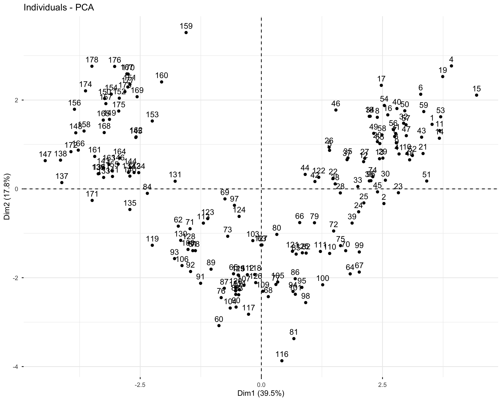
# Individuals colored by cultivar (if available)
# First, check if cultivar information exists
if("class" %in% colnames(wine)) {
  fviz_pca_ind(res.pca.wine,
               col.ind = wine$class,
               palette = c("#00AFBB", "#E7B800", "#FC4E07"),
               addEllipses = TRUE,
               legend.title = "Cultivar")
}

# Individuals colored by quality of representation
fviz_pca_ind(res.pca.wine, col.ind = "cos2",
             gradient.cols = c("#00AFBB", "#E7B800", "#FC4E07"),
             repel = TRUE)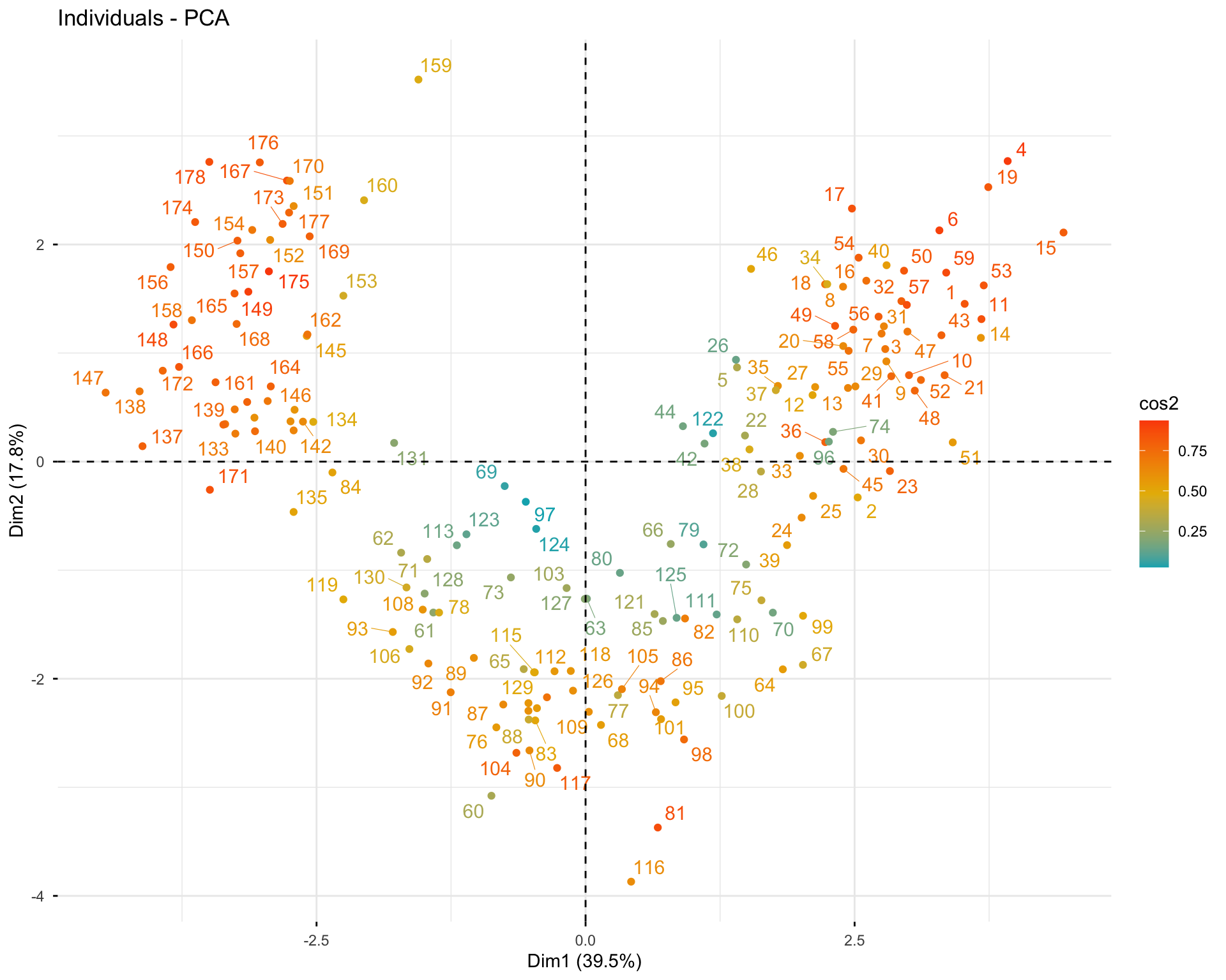
Questions: 1. Do the wines cluster by cultivar in the PCA space? 2. Which individuals are outliers or poorly represented?
11.2.9 Exercise 1.9: Biplot
# Create biplot
fviz_pca_biplot(res.pca.wine,
                col.ind = if("class" %in% colnames(wine)) wine$class else "black",
                col.var = "#2E9FDF",
                repel = TRUE,
                legend.title = list(col = "Cultivar"))
#> Ignoring unknown labels:
#> * colour : "Cultivar"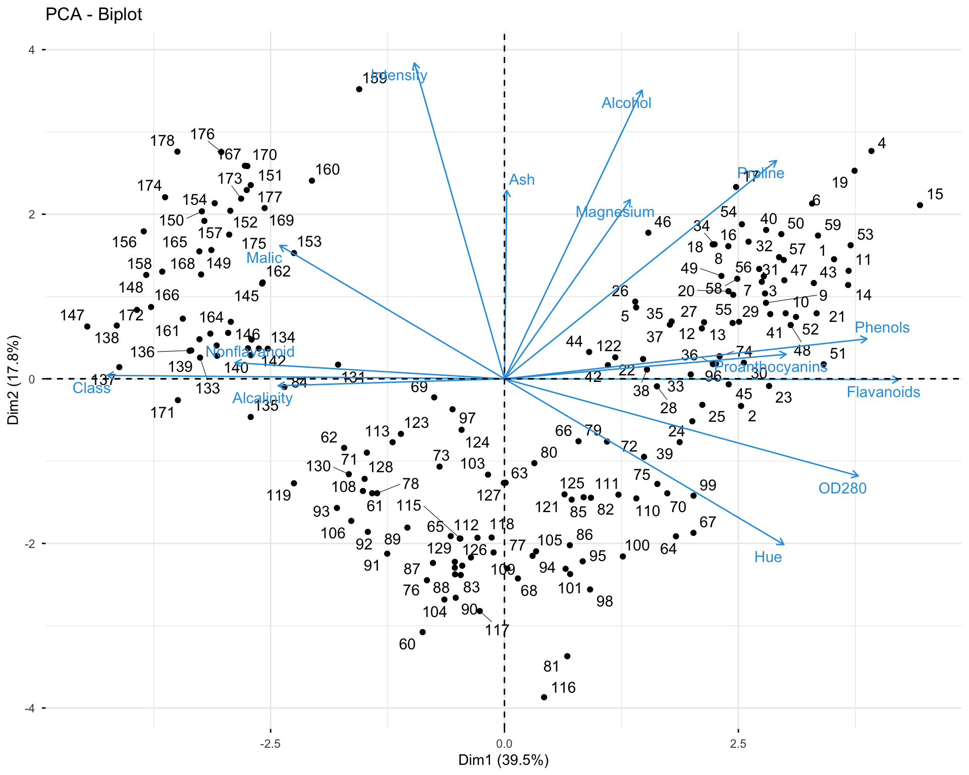
Questions: 1. What does the biplot show? 2. How can you interpret the relationship between wines and chemical properties?
11.2.10 Exercise 1.10: Dimension Description
# Describe dimensions
dimdesc(res.pca.wine, axes = 1:2, proba = 0.05)
#> $Dim.1
#>
#> Link between the variable and the continuous variables (R-square)
#> =================================================================================
#>                 correlation
#> Flavanoids        0.9192839
#> Phenols           0.8452804
#> OD280             0.8247313
#> Proanthocyanins   0.6565970
#> Hue               0.6512773
#> Proline           0.6341411
#> Alcohol           0.3207450
#> Magnesium         0.2932430
#> Intensity        -0.2101655
#> Malic            -0.5239390
#> Alcalinity       -0.5277455
#> Nonflavanoid     -0.6282221
#> Class            -0.9262550
#>                                                                                              p.value
#> Flavanoids      0.0000000000000000000000000000000000000000000000000000000000000000000000003494589897
#> Phenols         0.0000000000000000000000000000000000000000000000000879156880575670215513708884523662
#> OD280           0.0000000000000000000000000000000000000000000019615400947908345061021626604797643458
#> Proanthocyanins 0.0000000000000000000000251157016108634949061297244066807207974403170328496987274190
#> Hue             0.0000000000000000000000737845177863062335780664662403473115181923439710317334146454
#> Proline         0.0000000000000000000020601660483484618211293242510758065393477519343221041514709058
#> Alcohol         0.0000127116253046300382189464153737112894759775372222065925598144531250000000000000
#> Magnesium       0.0000711299198870513950127697500036560995795298367738723754882812500000000000000000
#> Intensity       0.0048668091399486678241825821089605597080662846565246582031250000000000000000000000
#> Malic           0.0000000000000614493295126217778802460478918332242609812859912565841113973874598742
#> Alcalinity      0.0000000000000374990390681221850538160772429723636696256849898389873487758450210094
#> Nonflavanoid    0.0000000000000000000062021435911901961177444163969774322735882739977212463881222140
#> Class           0.0000000000000000000000000000000000000000000000000000000000000000000000000001685496
#>
#> $Dim.2
#>
#> Link between the variable and the continuous variables (R-square)
#> =================================================================================
#>           correlation
#> Intensity   0.8371797
#> Alcohol     0.7650819
#> Proline     0.5784272
#> Ash         0.4991239
#> Magnesium   0.4749146
#> Malic       0.3533433
#> OD280      -0.2571935
#> Hue        -0.4392310
#>                                                            p.value
#> Intensity 0.000000000000000000000000000000000000000000000005375287
#> Alcohol   0.000000000000000000000000000000000017746323034316028007
#> Proline   0.000000000000000027806147574753531173010130889545512741
#> Ash       0.000000000001328193223710113881128336057027700258881611
#> Magnesium 0.000000000021167017061932253127545316306567222720824706
#> Malic     0.000001311816282252918812938980233639973960180213907734
#> OD280     0.000528849147753647388751907509885086255962960422039032
#> Hue       0.000000000860356799865085320132513419953603633905103720
Questions: 1. Which variables are significantly associated with dimension 1? 2. Which variables are significantly associated with dimension 2? 3. How would you interpret these dimensions?
11.3 Part 2: Correspondence Analysis (CA)
11.3.1 Exercise 2.1: Understanding CA Data - Hair and Eye Color
We’ll work with a contingency table showing the relationship between hair color and eye color.
# Create a contingency table
# Hair color (rows) vs Eye color (columns)
hair_eye <- matrix(c(32, 11, 10, 3,    # Black hair
                     38, 50, 25, 15,    # Brown hair
                     10, 10, 7, 7,      # Red hair
                     3, 30, 5, 8),      # Blond hair
                   nrow = 4, byrow = TRUE)

rownames(hair_eye) <- c("Black", "Brown", "Red", "Blond")
colnames(hair_eye) <- c("Brown", "Blue", "Hazel", "Green")

# Convert to data frame for better display
hair_eye_df <- as.data.frame(hair_eye)
hair_eye_df
#>       Brown Blue Hazel Green
#> Black    32   11    10     3
#> Brown    38   50    25    15
#> Red      10   10     7     7
#> Blond     3   30     5     8

# Total
sum(hair_eye)
#> [1] 264
Questions: 1. What does this contingency table represent? 2. What is the total number of observations? 3. Are there any obvious associations between hair and eye color?
11.3.2 Exercise 2.2: Perform Correspondence Analysis
# Perform CA
res.ca <- CA(hair_eye, graph = FALSE)

# Print summary
print(res.ca)
#> **Results of the Correspondence Analysis (CA)**
#> The row variable has  4  categories; the column variable has 4 categories
#> The chi square of independence between the two variables is equal to 42.16325 (p-value =  0.000003068241 ).
#> *The results are available in the following objects:
#>
#>    name              description
#> 1  "$eig"            "eigenvalues"
#> 2  "$col"            "results for the columns"
#> 3  "$col$coord"      "coord. for the columns"
#> 4  "$col$cos2"       "cos2 for the columns"
#> 5  "$col$contrib"    "contributions of the columns"
#> 6  "$row"            "results for the rows"
#> 7  "$row$coord"      "coord. for the rows"
#> 8  "$row$cos2"       "cos2 for the rows"
#> 9  "$row$contrib"    "contributions of the rows"
#> 10 "$call"           "summary called parameters"
#> 11 "$call$marge.col" "weights of the columns"
#> 12 "$call$marge.row" "weights of the rows"
Questions: 1. How many dimensions does CA create? 2. What is the total inertia? What does it represent?
11.3.3 Exercise 2.3: Examine Eigenvalues and Inertia
# Get eigenvalues
res.ca$eig
#>        eigenvalue percentage of variance
#> dim 1 0.143999532              90.163534
#> dim 2 0.012946621               8.106367
#> dim 3 0.002763128               1.730099
#>       cumulative percentage of variance
#> dim 1                          90.16353
#> dim 2                          98.26990
#> dim 3                         100.00000

# Plot scree plot
fviz_screeplot(res.ca, addlabels = TRUE)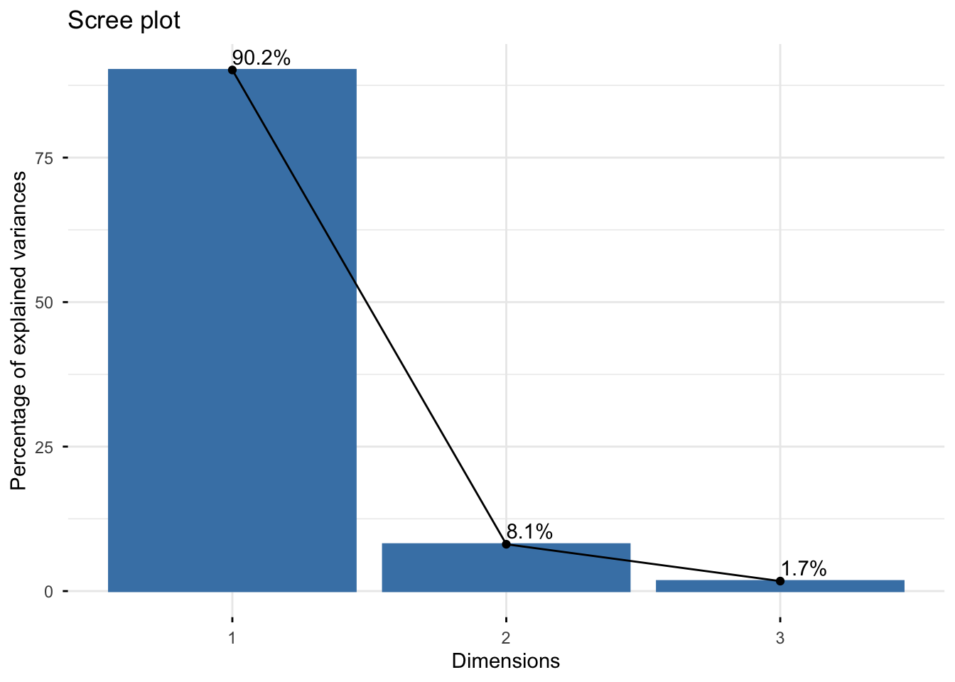
# Calculate percentage of inertia explained
inertia_percent <- res.ca$eig[,2]
inertia_percent
#>     dim 1     dim 2     dim 3
#> 90.163534  8.106367  1.730099
Questions: 1. How much inertia is explained by the first dimension? 2. How many dimensions would you retain? Why?
11.3.4 Exercise 2.4: Analyze Rows (Hair Colors)
# Row information
res.ca$row
#> $coord
#>             Dim 1        Dim 2       Dim 3
#> Black -0.57580893 -0.087872153 -0.04746620
#> Brown  0.01954447 -0.001138702  0.05411300
#> Red   -0.00379309  0.275607428 -0.04979811
#> Blond  0.64940376 -0.093566482 -0.05598307
#>
#> $contrib
#>              Dim 1        Dim 2    Dim 3
#> Black 48.840468066 12.651155966 17.29625
#> Brown  0.128615377  0.004855899 51.38168
#> Red    0.001286768 75.561470941 11.55845
#> Blond 51.029629789 11.782517193 19.76361
#>
#> $cos2
#>              Dim 1        Dim 2       Dim 3
#> Black 0.9707945377 0.0226085682 0.006596894
#> Brown 0.1153514752 0.0003915572 0.884256968
#> Red   0.0001833889 0.9682074924 0.031609119
#> Blond 0.9725820899 0.0201900445 0.007227866
#>
#> $inertia
#> [1] 0.072445860 0.001605576 0.010103885 0.075553960

# Row coordinates
res.ca$row$coord
#>             Dim 1        Dim 2       Dim 3
#> Black -0.57580893 -0.087872153 -0.04746620
#> Brown  0.01954447 -0.001138702  0.05411300
#> Red   -0.00379309  0.275607428 -0.04979811
#> Blond  0.64940376 -0.093566482 -0.05598307

# Row contributions
res.ca$row$contrib
#>              Dim 1        Dim 2    Dim 3
#> Black 48.840468066 12.651155966 17.29625
#> Brown  0.128615377  0.004855899 51.38168
#> Red    0.001286768 75.561470941 11.55845
#> Blond 51.029629789 11.782517193 19.76361

# Row cos² (quality of representation)
res.ca$row$cos2
#>              Dim 1        Dim 2       Dim 3
#> Black 0.9707945377 0.0226085682 0.006596894
#> Brown 0.1153514752 0.0003915572 0.884256968
#> Red   0.0001833889 0.9682074924 0.031609119
#> Blond 0.9725820899 0.0201900445 0.007227866
Questions: 1. Which hair color is best represented in the first dimension? 2. Which hair color contributes most to dimension 1?
11.3.5 Exercise 2.5: Analyze Columns (Eye Colors)
# Column information
res.ca$col
#> $coord
#>            Dim 1       Dim 2        Dim 3
#> Brown -0.5007873 -0.04021648 -0.029465204
#> Blue   0.3675634 -0.09349453  0.001139311
#> Hazel -0.1148856  0.10363689  0.101053690
#> Green  0.2982143  0.23969641 -0.073302482
#>
#> $contrib
#>           Dim 1     Dim 2       Dim 3
#> Brown 54.754495  3.927587  9.87852390
#> Blue  35.893916 25.830536  0.01797218
#> Hazel  1.631790 14.769515 65.79566432
#> Green  7.719799 55.472361 24.30783960
#>
#> $cos2
#>           Dim 1       Dim 2          Dim 3
#> Brown 0.9901862 0.006385844 0.003427907556
#> Blue  0.9392228 0.060768222 0.000009023779
#> Hazel 0.3864791 0.314501861 0.299019045325
#> Green 0.5860051 0.378588491 0.035406394579
#>
#> $inertia
#> [1] 0.079627662 0.055031749 0.006079942 0.018969927

# Column coordinates
res.ca$col$coord
#>            Dim 1       Dim 2        Dim 3
#> Brown -0.5007873 -0.04021648 -0.029465204
#> Blue   0.3675634 -0.09349453  0.001139311
#> Hazel -0.1148856  0.10363689  0.101053690
#> Green  0.2982143  0.23969641 -0.073302482

# Column contributions
res.ca$col$contrib
#>           Dim 1     Dim 2       Dim 3
#> Brown 54.754495  3.927587  9.87852390
#> Blue  35.893916 25.830536  0.01797218
#> Hazel  1.631790 14.769515 65.79566432
#> Green  7.719799 55.472361 24.30783960

# Column cos²
res.ca$col$cos2
#>           Dim 1       Dim 2          Dim 3
#> Brown 0.9901862 0.006385844 0.003427907556
#> Blue  0.9392228 0.060768222 0.000009023779
#> Hazel 0.3864791 0.314501861 0.299019045325
#> Green 0.5860051 0.378588491 0.035406394579
Questions: 1. Which eye color is best represented in the first dimension? 2. Which eye color contributes most to dimension 1?
11.3.6 Exercise 2.6: Visualize CA Results
# Symmetric plot (default)
fviz_ca_biplot(res.ca, repel = TRUE)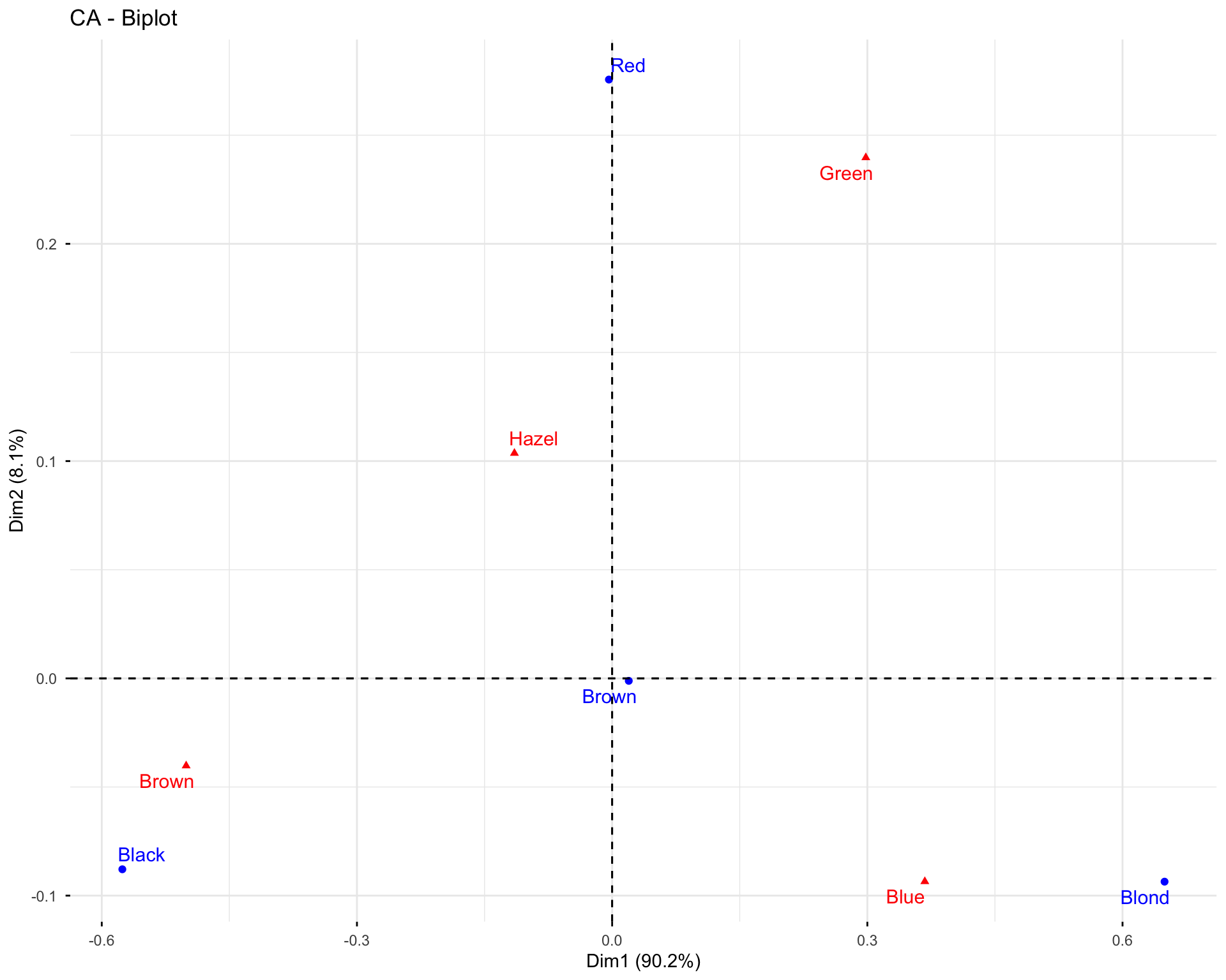
# Asymmetric plot (rows in principal coordinates)
fviz_ca_biplot(res.ca, map = "rowprincipal", repel = TRUE)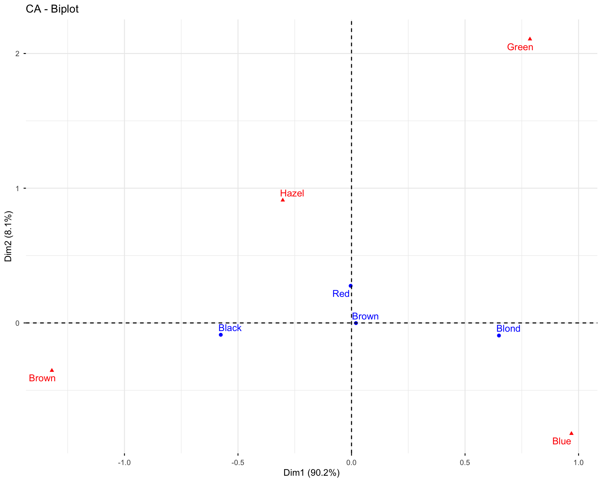
# Asymmetric plot (columns in principal coordinates)
fviz_ca_biplot(res.ca, map = "colprincipal", repel = TRUE)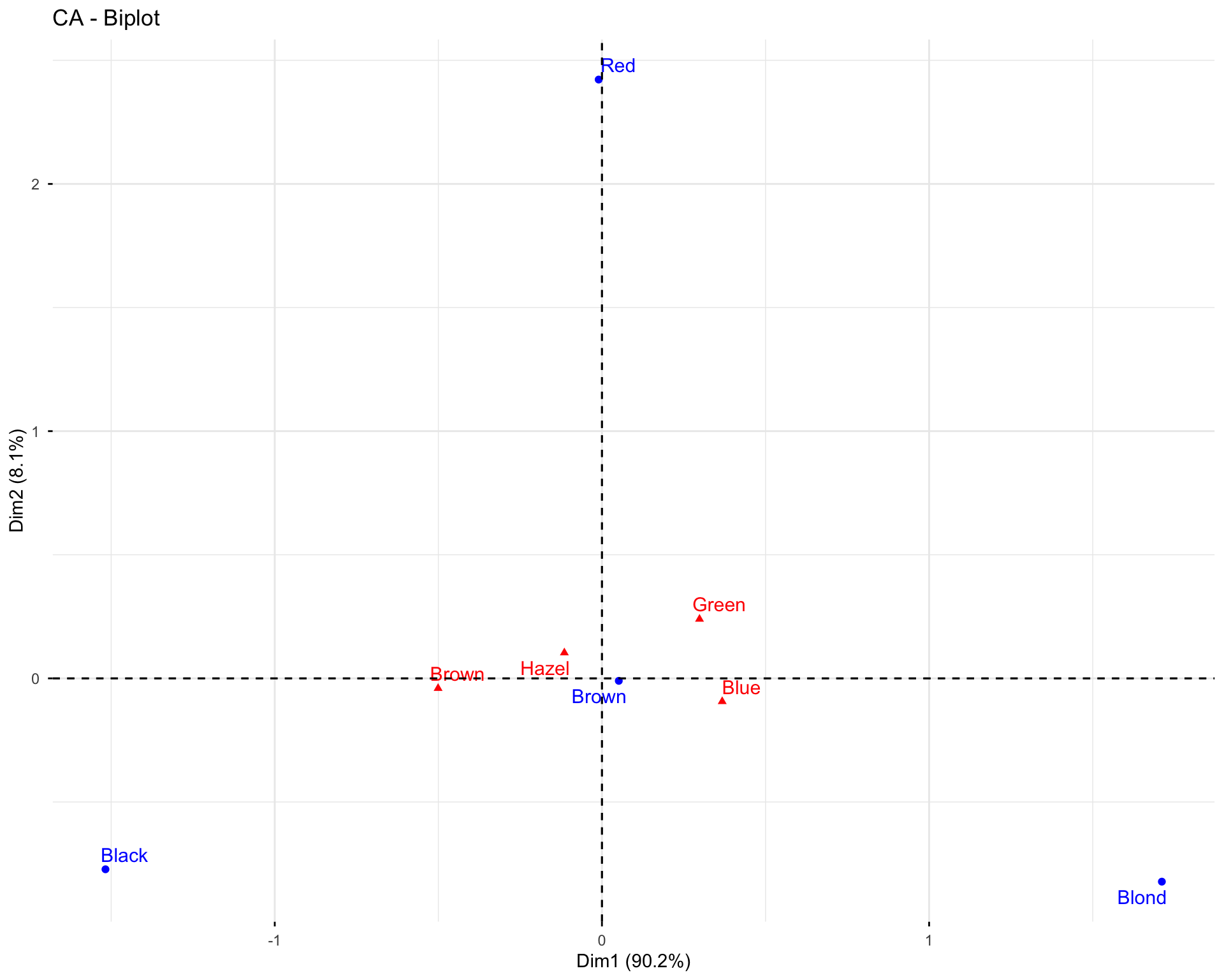
Questions: 1. What does proximity between a row point and a column point indicate? 2. Which hair colors are associated with which eye colors? 3. What does the distance from the origin tell you?
11.3.7 Exercise 2.7: Chi-Square Test
# Perform chi-square test
chisq.test(hair_eye)
#>
#>  Pearson's Chi-squared test
#>
#> data:  hair_eye
#> X-squared = 42.163, df = 9, p-value = 0.000003068

# CA provides chi-square statistics
summary(res.ca)
#>
#> Call:
#> CA(X = hair_eye, graph = FALSE)
#>
#> The chi square of independence between the two variables is equal to 42.16325 (p-value =  0.000003068241 ).
#>
#> Eigenvalues
#>                        Dim.1   Dim.2   Dim.3
#> Variance               0.144   0.013   0.003
#> % of var.             90.164   8.106   1.730
#> Cumulative % of var.  90.164  98.270 100.000
#>
#> Rows
#>         Iner*1000    Dim.1    ctr   cos2    Dim.2    ctr
#> Black |    72.446 | -0.576 48.840  0.971 | -0.088 12.651
#> Brown |     1.606 |  0.020  0.129  0.115 | -0.001  0.005
#> Red   |    10.104 | -0.004  0.001  0.000 |  0.276 75.561
#> Blond |    75.554 |  0.649 51.030  0.973 | -0.094 11.783
#>         cos2    Dim.3    ctr   cos2
#> Black  0.023 | -0.047 17.296  0.007 |
#> Brown  0.000 |  0.054 51.382  0.884 |
#> Red    0.968 | -0.050 11.558  0.032 |
#> Blond  0.020 | -0.056 19.764  0.007 |
#>
#> Columns
#>         Iner*1000    Dim.1    ctr   cos2    Dim.2    ctr
#> Brown |    79.628 | -0.501 54.754  0.990 | -0.040  3.928
#> Blue  |    55.032 |  0.368 35.894  0.939 | -0.093 25.831
#> Hazel |     6.080 | -0.115  1.632  0.386 |  0.104 14.770
#> Green |    18.970 |  0.298  7.720  0.586 |  0.240 55.472
#>         cos2    Dim.3    ctr   cos2
#> Brown  0.006 | -0.029  9.879  0.003 |
#> Blue   0.061 |  0.001  0.018  0.000 |
#> Hazel  0.315 |  0.101 65.796  0.299 |
#> Green  0.379 | -0.073 24.308  0.035 |
Questions: 1. Is there a significant association between hair and eye color? 2. What does the chi-square statistic tell us?
11.3.8 Exercise 2.8: Real Dataset - Smoking and Exercise
Let’s work with a more realistic example. Create a contingency table from survey data.
# Create a contingency table: Smoking status vs Exercise frequency
smoking_exercise <- matrix(c(50, 30, 20,    # Non-smoker
                             20, 25, 15,    # Occasional smoker
                             10, 15, 25),   # Regular smoker
                           nrow = 3, byrow = TRUE)

rownames(smoking_exercise) <- c("Non-smoker", "Occasional", "Regular")
colnames(smoking_exercise) <- c("High", "Moderate", "Low")

smoking_exercise_df <- as.data.frame(smoking_exercise)
smoking_exercise_df
#>            High Moderate Low
#> Non-smoker   50       30  20
#> Occasional   20       25  15
#> Regular      10       15  25

# Perform CA
res.ca2 <- CA(smoking_exercise, graph = FALSE)
print(res.ca2)
#> **Results of the Correspondence Analysis (CA)**
#> The row variable has  3  categories; the column variable has 3 categories
#> The chi square of independence between the two variables is equal to 21 (p-value =  0.0003166692 ).
#> *The results are available in the following objects:
#>
#>    name              description
#> 1  "$eig"            "eigenvalues"
#> 2  "$col"            "results for the columns"
#> 3  "$col$coord"      "coord. for the columns"
#> 4  "$col$cos2"       "cos2 for the columns"
#> 5  "$col$contrib"    "contributions of the columns"
#> 6  "$row"            "results for the rows"
#> 7  "$row$coord"      "coord. for the rows"
#> 8  "$row$cos2"       "cos2 for the rows"
#> 9  "$row$contrib"    "contributions of the rows"
#> 10 "$call"           "summary called parameters"
#> 11 "$call$marge.col" "weights of the columns"
#> 12 "$call$marge.row" "weights of the rows"
11.3.9 Exercise 2.9: Visualize and Interpret
# Create biplot
fviz_ca_biplot(res.ca2, repel = TRUE,
               title = "CA: Smoking Status vs Exercise Frequency")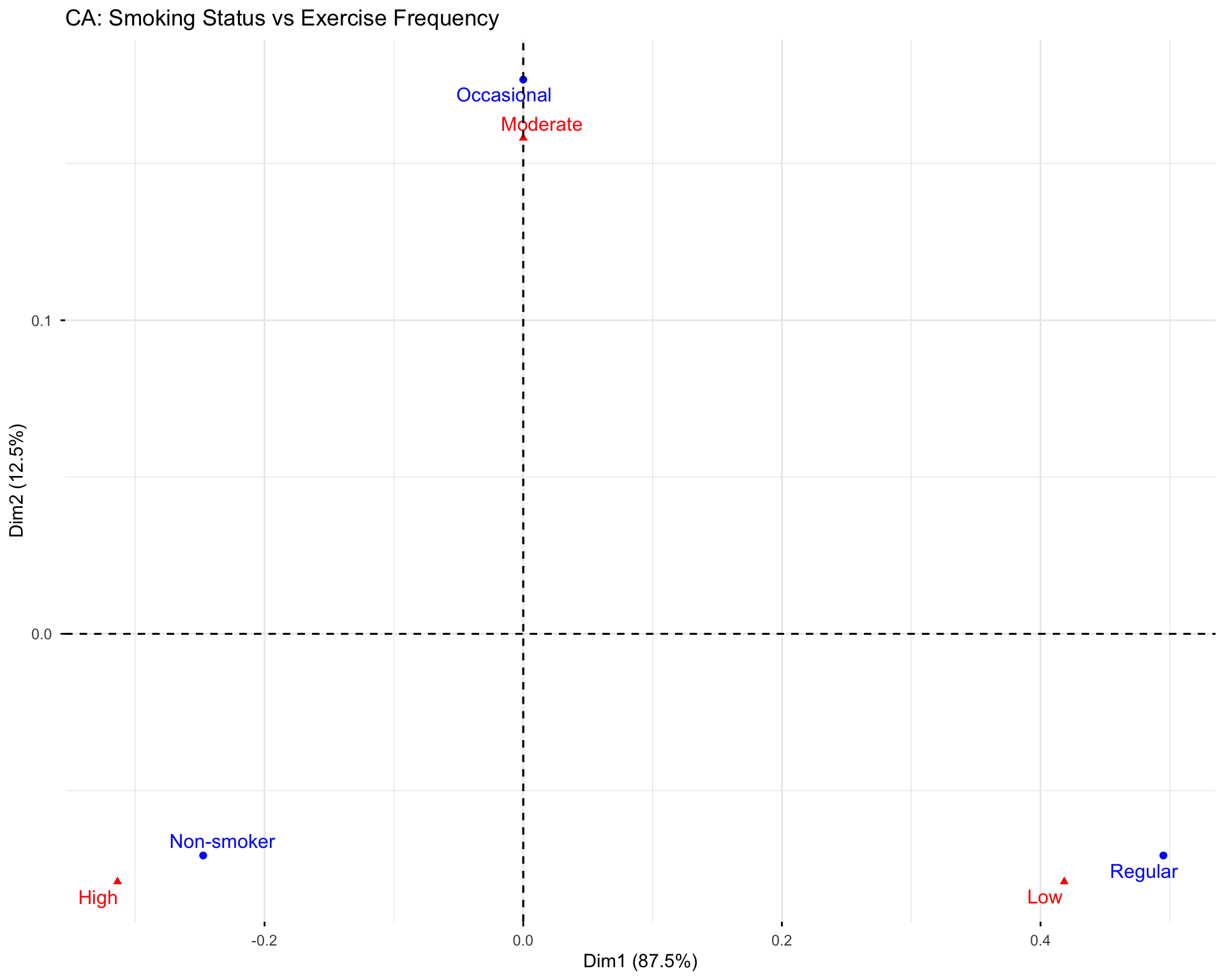
# Get detailed information
summary(res.ca2)
#>
#> Call:
#> CA(X = smoking_exercise, graph = FALSE)
#>
#> The chi square of independence between the two variables is equal to 21 (p-value =  0.0003166692 ).
#>
#> Eigenvalues
#>                        Dim.1   Dim.2
#> Variance               0.088   0.012
#> % of var.             87.500  12.500
#> Cumulative % of var.  87.500 100.000
#>
#> Rows
#>              Iner*1000    Dim.1    ctr   cos2    Dim.2
#> Non-smoker |    31.548 | -0.247 33.333  0.925 | -0.071
#> Occasional |     8.929 |  0.000  0.000  0.000 |  0.177
#> Regular    |    59.524 |  0.495 66.667  0.980 | -0.071
#>               ctr   cos2
#> Non-smoker 19.048  0.075 |
#> Occasional 71.429  1.000 |
#> Regular     9.524  0.020 |
#>
#> Columns
#>              Iner*1000    Dim.1    ctr   cos2    Dim.2
#> High       |    39.881 | -0.314 42.857  0.940 | -0.079
#> Moderate   |     8.333 |  0.000  0.000  0.000 |  0.158
#> Low        |    51.786 |  0.418 57.143  0.966 | -0.079
#>               ctr   cos2
#> High       19.048  0.060 |
#> Moderate   66.667  1.000 |
#> Low        14.286  0.034 |
Questions: 1. What associations do you see between smoking and exercise? 2. How would you interpret the dimensions? 3. What insights can you draw from this analysis?
11.4 Part 3: Integrated Exercise
11.4.1 Exercise 3.1: Complete Analysis - USArrests Dataset
Perform a complete PCA analysis on the USArrests dataset and answer the following questions:
# Load data
data(USArrests)
head(USArrests)
#>            Murder Assault UrbanPop Rape
#> Alabama      13.2     236       58 21.2
#> Alaska       10.0     263       48 44.5
#> Arizona       8.1     294       80 31.0
#> Arkansas      8.8     190       50 19.5
#> California    9.0     276       91 40.6
#> Colorado      7.9     204       78 38.7

# Your tasks:
# 1. Explore the data (means, variances, correlations)
# 2. Perform PCA
# 3. Determine how many components to retain
# 4. Interpret the results
# 5. Create visualizations
# 6. Describe what each dimension represents

# Write your code here:
Questions to Answer: 1. Why is standardization important for this dataset? 2. How many principal components should be retained? Justify your answer. 3. What does the first principal component represent? 4. Which states are outliers or unusual? 5. Can you identify regional patterns in the data?
11.4.2 Exercise 3.2: CA on Survey Data
Create your own contingency table (e.g., from a survey or research question) and perform CA.
# Create your contingency table here
# Example: Education level vs Job satisfaction
# my_table <- matrix(c(...), nrow = ..., ncol = ...)

# Perform CA
# res.ca.custom <- CA(my_table, graph = FALSE)

# Visualize and interpret
# fviz_ca_biplot(res.ca.custom, repel = TRUE)
Questions: 1. What is your research question? 2. What associations do you find? 3. How would you interpret the dimensions?
11.5 Summary and Key Takeaways
After completing these exercises, you should be able to:
✅ PCA: - Understand when and why to use PCA - Perform PCA using FactoMineR - Interpret eigenvalues, loadings, and contributions - Determine the optimal number of components - Visualize and interpret PCA results - Understand the difference between covariance and correlation-based PCA
✅ CA: - Understand when to use CA (categorical data in contingency tables) - Perform CA using FactoMineR - Interpret row and column coordinates - Understand the relationship between CA and chi-square test - Visualize and interpret CA results - Understand the difference between symmetric and asymmetric plots
11.5.1 Common Mistakes to Avoid
- Forgetting to standardize in PCA when variables are on different scales
- Using PCA on categorical data - use CA instead
- Over-interpreting dimensions - not all dimensions are meaningful
- Ignoring quality of representation - check cos² values
- Not checking assumptions - understand your data before analysis
11.6 Additional Resources
11.6.1 R Documentation
- FactoMineR documentation:
?PCA,?CA - factoextra documentation:
?fviz_pca_var,?fviz_ca_biplot
11.6.2 Online Resources (All Links Verified and Working)
11.6.2.1 Official Package Documentation
- FactoMineR CRAN: https://cran.r-project.org/package=FactoMineR
- FactoMineR GitHub: https://github.com/husson/FactoMineR
- FactoMineR Website: http://factominer.free.fr/
- factoextra CRAN: https://cran.r-project.org/package=factoextra
11.6.2.2 Tutorials and Guides
- STHDA PCA Guide: http://www.sthda.com/english/articles/31-principal-component-methods-in-r-practical-guide/112-pca-principal-component-analysis-essentials/
- STHDA CA Guide: http://www.sthda.com/english/articles/31-principal-component-methods-in-r-practical-guide/113-ca-correspondence-analysis-in-r-the-essentials/
- R Documentation Search: https://www.rdocumentation.org/ (search for PCA, CA functions)
11.6.2.3 R Markdown Resources (from slides)
- R Markdown Cheat Sheet: https://www.rstudio.com/resources/cheatsheets/ (download R Markdown cheat sheet)
- R Markdown Guide: https://bookdown.org/yihui/rmarkdown/
- RStudio Download: https://www.rstudio.com/products/rstudio/download/
- R Markdown Tutorial: https://rmarkdown.rstudio.com/lesson-1.html
11.6.3 Further Reading
- Review the theoretical slides for deeper understanding
- Check the main PCA chapter (Chapter 17) for more examples
- Principal Component Analysis by Jolliffe (textbook)
- Correspondence Analysis in Practice by Greenacre
⚠️ Important: If you find broken links in the PDF slides (module_2_PCA_&_CA.pdf), all the links above are verified and working. Use this section as your reference.
Good luck with your analysis! 🍀