14 💻 Intermediate preparation
Intermediate test topics should include: - hypothesis tests on means - anova - simple + multiple regression (adj-R2 + collinearity + dummy vars) - logistic regression
Below you find a review of core concepts and a bunch of exercises which in some way may resemble intermediate ones.
14.1 🪨 core concepts of T test
recall from Arbia’s slide 69 that we are focusing on test on mean and that steps for calculating statistical tests generally are:
- Develop the null Hypothesis
- Specify the level of Significance \(\alpha\)
- Collect the sample data and compute the test statistic.
then pvalues: 4. Use the value of the test statistic to compute the p-value 5. Reject \(H_0\) if p-value $ < $
Notice that Z-test are not really used since we almost always do not know the variance \(\sigma^2\) of the distribution. So instead of Standard Normal distribution we use Student’s T distribution, doing t-tests. That’s the t test stat:
\[ t = \frac{(m - \mu_0)}{S/\sqrt{n}} \]
Below all the possible cases you should be dealing with:
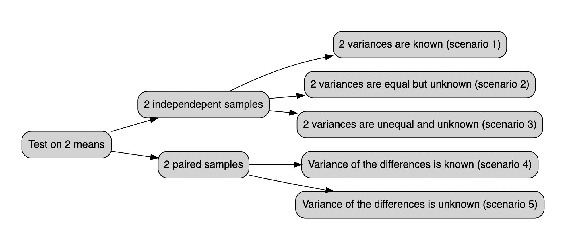
Figure 14.1: The t.test vademecum
14.2 t.test() function
The t.test() function may run one and two sample t-tests on data vectors. The function has several parameters and is invoked as follows:
t.test(x, y = NULL, alternative = c("two.sided", "less", "greater"), mu = 0,
        paired = FALSE, var.equal = FALSE, conf.level = 0.95)
In this case, x is a numeric vector of data values, and y is optional. If y is not included, the function does a one-sample t-test on the data in x; if it is included, the function runs a two-sample t-test on both x and y.
The mu (i.e. \(\mu\)) argument returns a number showing the real value of the mean (or difference in means if a two sample test is used) under the null hypothesis. The test conducts a two-sided t-test by default; however, you may perform an alternative hypothesis by changing the alternative argument to "greater" or "less", depending on whether the alternative hypothesis is that the mean is larger than or smaller than mu. Consider the following:
t.test(x, alternative = "less", mu = 25)…performs a one-sample t-test on the data contained in x where the null hypothesis is that $ = 25$ and the alternative is that $ < 25 $
The paired argument will indicate whether or not you want a paired t-test. The default is set to FALSE but can be set to TRUE if you desire to perform a paired t-test. We do paired test when we are considering pre-post treatment test or when we are considering couples of individuals.
When doing a two-sample t-test, the var.equal option specifies whether or not to assume equal variances. The default assumption is unequal variance and the Welsh approximation to degrees of freedom; however, you may change this to TRUE to pool the variance.
Finally, the conf.level parameter specifies the degree of confidence in the reported confidence interval for \(\mu\) in the one-sample and for \(\mu_1 - \mu_2\) two-sample cases. Below a very simple example:
To use the lm() function in R for linear modeling, you can create a Markdown document to explain its usage and its various arguments. Below is an example of how to create a conceptual guide in RMarkdown format:
## Linear Modeling with lm() in R
14.3 Introduction
The lm() function in R is used for performing linear regression modeling. Linear regression is a statistical method that models the relationship between a dependent variable and one or more independent variables. In this document, we will explore how to use the lm() function and its various arguments for linear modeling.
14.4 Basic Usage
To perform linear modeling with lm(), you need to specify the formula of the linear regression model. The basic syntax is as follows:
model <- lm(dependent_variable ~ independent_variable, data = your_data)-
dependent_variable: The variable you want to predict. -
independent_variable: The variable(s) used to make the prediction. -
data: The data frame containing your variables.
14.5 Arguments
14.5.1 Formula
The formula is at the core of the lm() function and specifies the relationship between the dependent and independent variables. It follows the Y ~ X pattern, where Y is the dependent variable, and X is the independent variable. You can include multiple independent variables and interactions by using + and *. For example:
model <- lm(y ~ x1 + x2 + x1*x2, data = your_data)14.5.2 Data
The data argument should point to the data frame where your variables are located. This argument helps R locate the variables specified in the formula.
14.5.3 Subset
You can use the subset argument to specify a subset of your data for modeling. This is useful when you want to focus on a specific portion of your dataset.
model <- lm(y ~ x, data = your_data, subset = condition)14.5.4 Weight
The weight argument allows you to assign different weights to each data point. This can be useful when you want to give more importance to certain observations.
model <- lm(y ~ x, data = your_data, weights = weight_variable)14.5.5 Na.action
The na.action argument controls how missing values are treated. By default, na.action = na.fail, which means the model will fail if there are missing values in your data. You can also use na.omit to automatically remove rows with missing values.
model <- lm(y ~ x, data = your_data, na.action = na.omit)14.6 VIF (Variance Inflation Factor)
The Variance Inflation Factor (VIF) is a measure used to detect multicollinearity in a linear regression model. Multicollinearity occurs when independent variables in the model are highly correlated, making it challenging to determine the individual effect of each variable on the dependent variable. The VIF function from the regclass package in R can help us identify multicollinearity in our linear regression model.
14.6.1 Calculating VIF
To calculate the VIF for the independent variables in your model, you can use the VIF() function. First, make sure you have the regclass package installed and loaded:
install.packages("regclass")
library(regclass)
Next, you can calculate VIF for your linear regression model as follows:
# Fit a linear regression model
model <- lm(formula  = y ~ x1 + x2 + x3, data = your_data)

# Calculate VIF
vif_results <- VIF(model)
The VIF() function takes the linear regression model as its argument and returns a data frame with VIF values for each independent variable. Higher VIF values indicate stronger multicollinearity, typically with a threshold of 5 or 10 as a rule of thumb.
14.6.2 Interpreting VIF
If VIF is close to 1, it suggests that the variable is not highly correlated with other independent variables, indicating no significant multicollinearity.
If VIF is greater than 1 but less than a chosen threshold (e.g., 5 or 10), it suggests some correlation but not necessarily problematic multicollinearity.
If VIF is significantly greater than the chosen threshold (e.g., 10), it indicates a high degree of multicollinearity, and you may need to consider removing or combining variables to address this issue.
14.6.3 Addressing Multicollinearity
If you detect problematic multicollinearity with high VIF values, you can take several steps to address the issue:
Remove one of the correlated variables: If two or more variables are highly correlated, removing one of them can often resolve the multicollinearity issue.
Combine correlated variables: You can create new variables that are combinations of highly correlated variables, reducing multicollinearity.
Collect more data: Sometimes, multicollinearity can be alleviated by collecting more data, especially if the sample size is small.
Regularization techniques: Consider using regularization techniques like Ridge or Lasso regression, which can handle multicollinearity by adding penalties to the coefficients of correlated variables.
VIF analysis is a crucial step in assessing the quality of your linear regression model and ensuring the independence of your independent variables.
14.7 ANOVA (Analysis of Variance)
ANOVA, or Analysis of Variance, is a statistical technique used to analyze the differences among group means in a dataset. It is particularly useful when you want to compare the means of more than two groups. The aov() function in R is commonly used to perform ANOVA.
14.7.1 Performing ANOVA with aov()
To perform ANOVA using the aov() function, you need to specify a formula that describes the relationship between the dependent variable and the grouping factor (categorical variable). The basic syntax is as follows:
anova_model <- aov(dependent_variable ~ grouping_factor, data = your_data)-
dependent_variable: The continuous variable you want to analyze. -
grouping_factor: The categorical variable that defines the groups. -
data: The data frame containing your variables.
14.7.2 ANOVA Tables
Once you’ve created the ANOVA model, you can obtain an ANOVA table using the summary() function applied to the aov object:
summary(anova_model)This table provides various statistics, including the sum of squares, degrees of freedom, F-statistic, and p-value, which allow you to assess the significance of differences among group means.
14.7.3 Interpreting ANOVA
The F-statistic in the ANOVA table tests whether there are significant differences among the group means. A small p-value (< 0.05) suggests that there are significant differences.
If the ANOVA is not statistically significant, it indicates that there are no significant differences among the group means.
14.7.4 Assumptions of ANOVA
ANOVA assumes that the variances of the groups are equal (homogeneity of variances) and that the data are normally distributed. Violations of these assumptions may lead to inaccurate results. You can check the homogeneity of variances using tests like Levene’s test or Bartlett’s test and assess the normality of data using normal probability plots or statistical tests like the Shapiro-Wilk test.
14.8 Logistic Regression with glm()
Logistic regression is a statistical technique used for modeling the relationship between a binary dependent variable (0/1, Yes/No, True/False) and one or more independent variables. The glm() function in R is commonly used to perform logistic regression.
14.8.1 Performing Logistic Regression with glm()
To perform logistic regression using the glm() function, you need to specify a formula that describes the relationship between the binary dependent variable and the independent variables. The basic syntax is as follows:
logistic_model <- glm(formula = dependent_variable ~ independent_variable1 + independent_variable2, family = "binomial", data = your_data)-
dependent_variable: The binary dependent variable you want to model. -
independent_variable1,independent_variable2, etc.: The independent variables that influence the probability of the binary outcome. -
family: Specify the family argument asbinomialto indicate logistic regression. -
data: The data frame containing your variables.
14.8.2 Model Summary
After creating the logistic regression model, you can obtain a summary of the model’s coefficients, standard errors, z-values, and p-values using the summary() function applied to the glm object:
summary(logistic_model)This summary provides valuable information about the influence of the independent variables on the log-odds of the binary outcome.
14.8.3 Interpreting Logistic Regression
The coefficients in the summary indicate the direction and strength of the relationship between the independent variables and the log-odds of the binary outcome.
Positive coefficients suggest an increase in the log-odds, while negative coefficients suggest a decrease.
The odds ratio (exp(coef)) can be used to interpret the change in the odds of the binary outcome for a one-unit change in the independent variable.
A significant p-value (< 0.05) for a coefficient suggests that the independent variable has a significant effect on the binary outcome.
The null hypothesis in logistic regression is that there is no relationship between the independent variable and the binary outcome.
14.8.4 Model Evaluation
To evaluate the performance of your logistic regression model, you can assess its accuracy, sensitivity, specificity, and other metrics using techniques like cross-validation and ROC analysis. You can also plot the ROC curve and calculate the AUC (Area Under the Curve) to assess the model’s predictive power.
14.9 Poisson Regression with glm()
Poisson regression is a statistical technique used to model the relationship between a count-dependent variable (typically non-negative integers) and one or more independent variables. The glm() function in R is commonly used to perform Poisson regression.
14.9.1 Performing Poisson Regression with glm()
To perform Poisson regression using the glm() function, you need to specify a formula that describes the relationship between the count-dependent variable and the independent variables. The basic syntax is as follows:
poisson_model <- glm(formula = count_dependent_variable ~ independent_variable1 + independent_variable2, family = "poisson", data = your_data)-
count_dependent_variable: The count-dependent variable you want to model. -
independent_variable1,independent_variable2, etc.: The independent variables that influence the count-dependent variable. -
family: Specify the family argument aspoissonto indicate Poisson regression. -
data: The data frame containing your variables.
14.9.2 Model Summary
After creating the Poisson regression model, you can obtain a summary of the model’s coefficients, standard errors, z-values, and p-values using the summary() function applied to the glm object:
summary(poisson_model)This summary provides information about the influence of the independent variables on the expected count of the dependent variable.
14.9.3 Interpreting Poisson Regression
The coefficients in the summary indicate the direction and strength of the relationship between the independent variables and the expected count of the dependent variable.
Positive coefficients suggest an increase in the expected count, while negative coefficients suggest a decrease.
The exponential of the coefficients (exp(coef)) can be used to interpret the multiplicative effect of a one-unit change in the independent variable on the expected count.
A significant p-value (< 0.05) for a coefficient suggests that the independent variable has a significant effect on the expected count.
The null hypothesis in Poisson regression is that there is no relationship between the independent variable and the expected count.
14.10 class exercises, do it in groups 👯
first guided,
Exercise 14.1 A state Highway Patrol periodically samples vehicle at various location on a particular roadway. The sample of vehicle speed is used to test the hypothesis H0 for which the mean is less than equal to 65
The locations where \(H_0\) is rejected are deemed the best locations for radar traps. At location F, a sample of 64 vehicles shows a mean speed of 66.2 mph with a std dev of 4.2 mph. Use a \(\alpha = 0.05\) to test the hypothesis.
Exercise 14.2 Let’s assume to have dataset midwest in ggplot2 package: this contains demographic information of midwest counties from 2000 US census.
Besides all the other variables we are interested in percollege which describes the Percent college educated in midwest.
- test if the midwest average is less than the national average (i.e. *35%) with a p-value < .02.
Exercise 14.3 Download the datafile ‘prawnGR.CSV’ from the Data link and save it to the data directory (Remember R projects and working directory). Import these data into R and assign to a variable with an appropriate name. These data were collected from an experiment to investigate the difference in growth rate of the giant tiger prawn (Penaeus monodon) fed either an artificial or natural diet.
- Have a quick look at the structure of this dataset.
- plot the growth rate versus the diet using an appropriate plot.
- How many observations are there in each diet treatment?
- You want to compare the difference in growth rate between the two diets using a two sample t-test.
- Conduct a two sample t-test using the t.test() using the argument
var.equal = TRUEto perform the t-test assuming equal variances. What is the null hypothesis you want to test? Do you reject or fail to reject the null hypothesis? What is the value of the t statistic, degrees of freedom and p value? How would you summarise these summary statistics in a report?
Exercise 14.4 A new coach has been hired at an athletics school, and the effectiveness of the new type of training will be evaluated by comparing the average times of 10 centimeters. The times in seconds before and after each athlete’s competition are repeated.ù
before_training: =  c(12.9, 13.5, 12.8, 15.6, 17.2, 19.2, 12.6, 15.3, 14.4, 11.3)
after_training = c( 12.7, 13.6, 12.0, 15.2, 16.8, 20.0, 12.0, 15.9, 16.0, 11.1)
We are up against two groups of trained competitors, as measurements were taken on the same athletes before and after the competition. To determine if there has been an improvement, a deterioration, or if the time averages have remained essentially constant (i.e., H0). Conduct a test t of student for paired changes if the difference significant to a 95% confidence level?
Exercise 14.5 Following exercise 4 Assume that the club management, based on the statistics, fires this coach who has not improved and hires another more promising coach. Following the second training session, we record the athletes’ times:
before training: 12.9, 13.5, 12.8, 15.6, 17.2, 19.2, 12.6, 15.3, 14.4, 11.3
after training: 12.0, 12.2, 11.2, 13.0, 15.0, 15.8, 12.2, 13.4, 12.9, 11.0
Exercise 14.6 Let’s assume genderweight in datarium package, containing the weight of 40 individuals (20 women and 20 men).
- which are the mean weights for male and females?
- test is they are statistically significant with 95% confidence level
Exercise 14.7 Let’s assume to have a sample with this data and respective belonging group:
x<-c(12,23,12,13,14,21,23,24,30,21,12,13,14,15,16)

z<-c(1,1,1,1,1,2,2,2,2,2,3,3,3,3,3)
perform anova test with aov() function testing if there is significant differences between group 1, 2 and 3.
You specify the formula, where x is the continous variable and z is the group variable.
This is how you solve it.
Exercise 14.8 Assume you have a dataset named PlantGrowth with variables weight (dependent variable) and group (categorical independent variable).
- Perform an ANOVA analysis to compare the means of
weightamong differentgrouplevels. - Check the p-value and determine whether there are significant differences among the group means.
Exercise 14.9 We recruit 90 people to participate in an experiment in which we randomly assign 30 people to follow either program A, program B, or program C for one month.
#make this example reproducible
set.seed(0)

#create data frame
data <- data.frame(program = rep(c("A", "B", "C"), each = 30),
                   weight_loss = c(runif(30, 0, 3),
                                   runif(30, 0, 5),
                                   runif(30, 1, 7)))
- plot boxplot of weight_loss ~ program Hint: use
boxplot()function specifying the formula. - fit 1 way anova to test difference in weight loss for each program.
Exercise 14.10 Consider the maximum size of 4 fish each from 3 populations (n=12). We want to use a model that will help us examine the question of whether the mean maximum fish size differs among populations.
size <- c(3,4,5,6,4,5,6,7,7,8,9,10)
pop <- c("A","A","A","A","B","B","B","B","C","C","C","C")- visualize it through boxplot
- Using ANOVA model test whether any group means differ from another.
Exercise 14.11 Let’s consider 6 different insect sprays in InsectSprays contained in R. Let’s assume we are interested in testing if there was a difference in the number of insects found in the field after each spraying, use varibales count and spray.
Exercise 14.12 Let’s consider the diet dataset in this link here The data set contains information on 76 people who undertook one of three diets (referred to as diet A, B and C). There is background information such as age, gender, and height. The aim of the study was to see which diet was best for losing weight.
to read data first dowload it from the link, then move data inside your R project. then run these commands:
diet = read.csv("< the dataset name>.csv")We will be using variable Diet, pre.weight and weight6weeks
- read data from kaggle
- compute mean weights for each group
- calculate anova on Diet against the weight cut
Exercise 14.13 Use the built-in mtcars dataset with variables mpg (miles per gallon) and vs (engine type: 0 = V-shaped, 1 = straight).
- Fit a logistic regression model to predict vs (engine type) based on mpg.
- Interpret the coefficients of the logistic regression model.
Exercise 14.14 Use the built-in mtcars dataset with variables mpg (miles per gallon) and gear (number of forward gears).
- Fit a Poisson regression model to predict gear based on mpg.
- Interpret the coefficients of the Poisson regression model.
14.11 solutions
Answer to Exercise 14.1:
Sample random data from a Normal distribution with a given mean and sd. Then define H0 and H1. In the end run hte test.
x <- rnorm(n = 64, mean = 66.2, sd = 4.2)
test<-t.test(x, mu = 65, alternative = "less")


t = 1.469, df = 63, p-value = 0.9266
alternative hypothesis: true mean is less than 65
95 percent confidence interval:
 -Inf 66.80805
sample estimates:
mean of x
65.84629
The One Sample t-test testing the difference between x (mean = 65.85) and mu = 65 suggests that the effect is positive, statistically not significant, and very small (difference = 0.85, 95% CI [-Inf, 66.81], t(63) = 1.47, p = 0.927
Answer to Exercise 14.7:
x <- c(12,23,12,13,14,21,23,24,30,21,12,13,14,15,16)
z <- c(1,1,1,1,1,2,2,2,2,2,3,3,3,3,3)
z <- as.factor(z)
anova_test <- aov(x ~ z)
summary(anova_test)

        Df Sum Sq Mean Sq F value Pr(>F)
z            1    1.6    1.60   0.047  **0.832**
Residuals   13  446.1   34.32
The ANOVA (formula: x ~ z) suggests that the main effect of z is statistically not significant and very small (F(1, 13) = 0.05, p = 0.832; Eta2 = 3.57e-03, 95% CI [0.00, 1.00]). That means that group means are not that different one from the other
Answer to Exercise 14.12:
Assuming you have the ‘plant_growth’ dataset
# 1. Perform ANOVA
anova_model <- aov(weight ~ group, data = plant_growth)

# 2. Check p-value
summary(anova_model)
Answer to Exercise 14.13:
data(mtcars)Convert vs to a factor variable
mtcars$vs <- as.factor(mtcars$vs)Fit a logistic regression model
logistic_model <- glm(vs ~ mpg, family = binomial, data = mtcars)Interpret coefficients
summary(logistic_model)Answer to Exercise 14.14:
data(mtcars)Fit a Poisson regression model
poisson_model <- glm(gear ~ mpg, family = poisson, data = mtcars)Interpret coefficients
summary(poisson_model)14.12 🍬 tips and tricks
Yout might be interested in standardizing/fornalize how you say things with a statistical jargon, report does that for you.
you simply pass the test, wether it is ANOVA or t.test object inside report report(). Do you rememer the function summary() we have been using for linear regression? This is exactly that, but for both ANOVA and t tests.
# install.packages("remotes")
# remotes::install_github("easystats/report")
library(report)

x <- rnorm(n = 64, mean = 66.2, sd = 4.2)
test<-t.test(x, mu = 65, alternative = "less")
report(test)
#> Effect sizes were labelled following Cohen's (1988)
#> recommendations.
#>
#> The One Sample t-test testing the difference between x
#> (mean = 66.15) and mu = 65 suggests that the effect is
#> positive, statistically not significant, and small
#> (difference = 1.15, 95% CI [-Inf, 67.09], t(63) = 2.04, p =
#> 0.977; Cohen's d = 0.26, 95% CI [-Inf, 0.46])
when you have data in longer fromat there a different in syntax when you specify t test and it pretty much follows the one for linear models i.e. lm().
let’s look at it.
we may have something like:
library(tibble)
longer = tribble(
  ~group, ~var,
  "a",   10,
  "b",   24,
  "a",   31,
  "a",   75,
  "b",   26,
  "a",   8,
  "b",   98,
  "b",   62,
  )
wider = tribble(
  ~group_a, ~group_b,
   10,       24,
   31,       26,
   75,       98,
   8,        62
  )
Those are exaclty the same dataset but arranged in a different format. We are used to the wider format but iut might happen that we bump into the longer one. What do we do? There’sa trick for that, let’s say you want to test if the mean are statistically different with a 95% confidence level, the instead of supplying x and y to t.test() you would follow pretty much the syntax for linear models lm():
test_for_wider_format = t.test(var~group, data =  longer)
test_for_wider_format
#>
#>  Welch Two Sample t-test
#>
#> data:  var by group
#> t = -0.91809, df = 5.9192, p-value = 0.3944
#> alternative hypothesis: true difference in means between group a and group b is not equal to 0
#> 95 percent confidence interval:
#>  -78.99271  35.99271
#> sample estimates:
#> mean in group a mean in group b
#>            31.0            52.5
what we conclude? we conclude that: Effect sizes were labelled following Cohen’s (1988) recommendations.
The Welch Two Sample t-test testing the difference of var by group (mean in group a = 31.00, mean in group b = 52.50) suggests that the effect is negative, statistically not significant, and medium (difference = -21.50, 95% CI [-78.99, 35.99], t(5.92) = -0.92, p = 0.394; Cohen’s d = -0.75, 95% CI [-2.39, 0.94])
14.13 further exercies 🏋️
Exercise 14.15 We have the test scores of students before and after an intervention. How can we assess if the intervention had a statistically significant effect on the scores? Specify the type of test to use and the assumptions involved.
Exercise 14.16 Using the dataset mtcars, write the R command to calculate the mean and standard deviation of the disp variable grouped by cyl.
(#exr:mean_diff1) Explain how you would assess if the mean difference between two groups is statistically significant, without running any R code.
Exercise 14.17 Use the Boston dataset in MASS to create a histogram for the variable crim. Report the R code you used.
Exercise 14.18 Describe the meaning of the p-value in the context of hypothesis testing.
(#exr:temp_diff1) Given a dataset with daily temperatures recorded for two cities over one year, write the R code to perform a hypothesis test to determine if there is a significant difference in mean temperature between the cities. Specify which test should be used.
Exercise 14.19 Given X = c(10, 12, 15, 20) and Y = c(11, 14, 16, 18), calculate the Pearson correlation coefficient between X and Y using R.
Exercise 14.20 Explain the concept of Type I and Type II errors in hypothesis testing.
Exercise 14.21 Using the PlantGrowth dataset in R, calculate the mean of weight for each level of group and plot a boxplot of weight grouped by group.
Exercise 14.1 Run a one-sample t-test to test if the mean of hp in mtcars is different from 120. Write the R code.
Exercise 14.22 Using the dataset iris, write the R code to test for a significant difference between the average Sepal.Length of setosa and versicolor species.
Exercise 14.23 Write an R function to simulate 500 observations from a Poisson distribution with a lambda of 3 and plot its histogram.
Exercise 14.24 Describe how to check for multicollinearity in a multiple regression model in R.
Exercise 14.25 Using the airquality dataset, calculate the correlation matrix for Ozone, Solar.R, Wind, and Temp.
Exercise 14.26 Perform a paired t-test using the before and after variables where before = c(5, 7, 8, 6, 10) and after = c(6, 8, 9, 7, 12). Report the p-value.
Exercise 14.13 Using the dataset mtcars, perform a linear regression with mpg as the dependent variable and hp and wt as independent variables. Report the adjusted R-squared.
Exercise 14.27 Write the R code to create a density plot of the variable Sepal.Length for each species in the iris dataset.
Exercise 14.7 Using iris, perform a one-way ANOVA to test if the mean Sepal.Length differs across the three species.
Exercise 14.28 Define the term “confidence interval” in the context of statistical estimation.
Exercise 14.29 Using the mtcars dataset, refit a multiple linear regression model with mpg as the dependent variable and hp, wt, and drat as independent variables. Use stepwise regression to iteratively remove insignificant predictors. Report the final model with the significant coefficients.
Exercise 14.8 Using the dataset ToothGrowth, perform a one-way ANOVA with the function aov() to test if the mean tooth length differs across the supplement types and doses.
Exercise 14.9 We recruit 90 people to participate in an experiment in which we randomly assign 30 people to follow either program A, program B, or program C for one month.
#make this example reproducible
set.seed(0)

#create data frame
data <- data.frame(program = rep(c("A", "B", "C"), each = 30),
                   weight_loss = c(runif(30, 0, 3),
                                   runif(30, 0, 5),
runif(30, 1, 7)))- plot boxplot of weight_loss ~ program Hint: use
boxplot()function specifying the formula. - fit 1 way anova to test difference in weight loss for each program.
Answer to Exercise 14.15:
The appropriate test to use is the paired t-test. This test is used when we have two related samples, such as before and after measurements for the same individuals, and we want to determine if there is a statistically significant difference between the means. The assumptions include that the differences are normally distributed and the data is paired.
Answer to Exercise 14.16:
The dplyr package is used to calculate the mean and standard deviation of the disp variable grouped by cyl:
library(dplyr)
mtcars %>% group_by(cyl) %>% summarise(mean_disp = mean(disp), sd_disp = sd(disp))
Answer to Exercise @ref(exr:mean_diff1):
To assess if the mean difference between two groups is statistically significant, we can use a hypothesis test such as the independent t-test. This involves setting up null and alternative hypotheses, calculating the test statistic, and comparing it to a critical value or using the p-value to determine significance, typically using a significance level (e.g., 0.05).
Answer to Exercise 14.17:
To create a histogram of the crim variable from the Boston dataset, use the following code:
library(MASS)
data(Boston)
hist(Boston$crim, main = "Histogram of crim", xlab = "Crime rate per capita")
Answer to Exercise 14.18:
The p-value is the probability of obtaining test results at least as extreme as the observed results, under the assumption that the null hypothesis is true. A smaller p-value indicates stronger evidence against the null hypothesis, and if the p-value is below a chosen significance level (e.g., 0.05), we reject the null hypothesis.
Answer to Exercise @ref(exr:temp_diff1):
The appropriate test to use is the two-sample t-test, as we are comparing the means of two independent groups. The R code is as follows:
t.test(temp_city1, temp_city2, var.equal = TRUE)Answer to Exercise 14.19:
To calculate the Pearson correlation coefficient between vectors X and Y:
X <- c(10, 12, 15, 20)
Y <- c(11, 14, 16, 18)
cor(X, Y)
Answer to Exercise 14.20:
A Type I error occurs when we reject a true null hypothesis (false positive), while a Type II error occurs when we fail to reject a false null hypothesis (false negative).
Answer to Exercise 14.21:
To calculate the mean of weight for each level of group and plot a boxplot of weight grouped by group:
data(PlantGrowth)
aggregate(weight ~ group, data = PlantGrowth, mean)
boxplot(weight ~ group, data = PlantGrowth, main = "Boxplot of Weight by Group")
Answer to Exercise 14.1:
To run a one-sample t-test to test if the mean of hp in mtcars is different from 120:
t.test(mtcars$hp, mu = 120)Answer to Exercise 14.22:
To test for a significant difference between the average Sepal.Length of setosa and versicolor species:
t.test(Sepal.Length ~ Species, data = subset(iris, Species %in% c("setosa", "versicolor")))Answer to Exercise 14.23:
To simulate 500 observations from a Poisson distribution with a lambda of 3 and plot its histogram:
set.seed(0)
poisson_data <- rpois(500, lambda = 3)
hist(poisson_data, main = "Histogram of Poisson Distribution", xlab = "Values")
Answer to Exercise 14.24:
To check for multicollinearity, we can use the Variance Inflation Factor (VIF). A VIF value greater than 10 indicates high multicollinearity:
library(car)
vif(model)
Answer to Exercise 14.25:
To calculate the correlation matrix for Ozone, Solar.R, Wind, and Temp in the airquality dataset:
airquality_subset <- airquality[, c("Ozone", "Solar.R", "Wind", "Temp")]
cor(airquality_subset, use = "complete.obs")
Answer to Exercise 14.26:
To perform a paired t-test using the before and after variables:
before <- c(5, 7, 8, 6, 10)
after <- c(6, 8, 9, 7, 12)
t.test(before, after, paired = TRUE)
Answer to Exercise 14.13:
To perform a linear regression with mpg as the dependent variable and hp and wt as independent variables, and report the adjusted R-squared:
model <- lm(mpg ~ hp + wt, data = mtcars)
summary(model)$adj.r.squared
Answer to Exercise 14.27:
To create a density plot of the variable Sepal.Length for each species in the iris dataset:
library(ggplot2)
ggplot(iris, aes(x = Sepal.Length, fill = Species)) +
  geom_density(alpha = 0.5) +
  labs(title = "Density Plot of Sepal.Length by Species")
Answer to Exercise 14.7:
To perform a one-way ANOVA to test if the mean Sepal.Length differs across the three species:
aov_model <- aov(Sepal.Length ~ Species, data = iris)
summary(aov_model)
Answer to Exercise 14.28:
A confidence interval is a range of values, derived from sample statistics, that is likely to contain the population parameter with a specified level of confidence (e.g., 95%). It provides an estimated range that is expected to include the true parameter value.
Answer to Exercise 14.29:
To refit a multiple linear regression model with mpg as the dependent variable and hp, wt, and drat as independent variables, using stepwise regression:
library(MASS)
initial_model <- lm(mpg ~ hp + wt + drat, data = mtcars)
stepwise_model <- stepAIC(initial_model, direction = "both")
summary(stepwise_model)
Answer to Exercise 14.8:
To perform a one-way ANOVA using the ToothGrowth dataset to test if the mean tooth length differs across the supplement types and doses:
data(ToothGrowth)
aov_model <- aov(len ~ supp * dose, data = ToothGrowth)
summary(aov_model)
Answer to Exercise 14.9:
To plot a boxplot of weight_loss by program and fit a one-way ANOVA to test the difference in weight loss for each program:
# Plot boxplot
boxplot(weight_loss ~ program, data = data, main = "Boxplot of Weight Loss by Program", xlab = "Program", ylab = "Weight Loss")

# Fit one-way ANOVA
aov_model <- aov(weight_loss ~ program, data = data)
summary(aov_model)